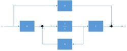
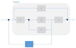
Full state feedback
Full state feedback (FSF), or pole placement, is a method employed in feedback control system theory to place the closed-loop poles of a plant in pre-determined locations in the s-plane.[1] Placing poles is desirable because the location of the poles corresponds directly to the eigenvalues of the system, which control the characteristics of the response of the system. The system must be considered controllable in order to implement this method.
Principle
If the closed-loop dynamics can be represented by the state space equation (see State space (controls))
- [math]\displaystyle{ \dot{\underline{x}}=\mathbf{A}\underline{x}+\mathbf{B}\underline{u}, }[/math]
with output equation
- [math]\displaystyle{ \underline{y} = \mathbf{C}\underline{x}+\mathbf{D}\underline{u}, }[/math]
then the poles of the system transfer function are the roots of the characteristic equation given by
- [math]\displaystyle{ \left|s\textbf{I}-\textbf{A}\right|=0. }[/math]
Full state feedback is utilized by commanding the input vector [math]\displaystyle{ \underline{u} }[/math]. Consider an input proportional (in the matrix sense) to the state vector,
- [math]\displaystyle{ \underline{u}=-\mathbf{K}\underline{x} }[/math].
Substituting into the state space equations above, we have
- [math]\displaystyle{ \dot{\underline{x}}=(\mathbf{A}-\mathbf{B}\mathbf{K})\underline{x} }[/math]
- [math]\displaystyle{ \underline{y} = (\mathbf{C}-\mathbf{D}\mathbf{K})\underline{x}. }[/math]
The poles of the FSF system are given by the characteristic equation of the matrix [math]\displaystyle{ \mathbf{A} - \mathbf{B}\mathbf{K} }[/math], [math]\displaystyle{ \det\left[s\textbf{I}-\left(\textbf{A}-\textbf{B}\textbf{K}\right)\right]=0 }[/math]. Comparing the terms of this equation with those of the desired characteristic equation yields the values of the feedback matrix [math]\displaystyle{ \textbf{K} }[/math] which force the closed-loop eigenvalues to the pole locations specified by the desired characteristic equation.[2]
Example of FSF
Consider a system given by the following state space equations:
- [math]\displaystyle{ \dot{\underline{x}}=\begin{bmatrix}0 & 1 \\ -2 & -3\end{bmatrix}\underline{x}+\begin{bmatrix} 0 \\ 1\end{bmatrix}\underline{u}. }[/math]
The uncontrolled system has open-loop poles at [math]\displaystyle{ s=-1 }[/math] and [math]\displaystyle{ s=-2 }[/math]. These poles are the eigenvalues of the [math]\displaystyle{ \mathbf{A} }[/math] matrix and they are the roots of [math]\displaystyle{ \left|s\mathbf{I} - \mathbf{A}\right| }[/math]. Suppose, for considerations of the response, we wish the controlled system eigenvalues to be located at [math]\displaystyle{ s=-1 }[/math] and [math]\displaystyle{ s=-5 }[/math], which are not the poles we currently have. The desired characteristic equation is then [math]\displaystyle{ s^2+6s+5=0 }[/math], from [math]\displaystyle{ (s + 1)(s + 5) }[/math].
Following the procedure given above, the FSF controlled system characteristic equation is
- [math]\displaystyle{ \left|s\mathbf{I}-\left(\mathbf{A}-\mathbf{B}\mathbf{K}\right)\right|=\det\begin{bmatrix}s & -1 \\ 2+k_1 & s+3+k_2 \end{bmatrix}=s^2+(3+k_2)s+(2+k_1), }[/math]
where
- [math]\displaystyle{ \mathbf{K}=\begin{bmatrix} k_1 & k_2\end{bmatrix}. }[/math]
Upon setting this characteristic equation equal to the desired characteristic equation, we find
- [math]\displaystyle{ \mathbf{K}=\begin{bmatrix}3 & 3\end{bmatrix} }[/math].
Therefore, setting [math]\displaystyle{ \underline{u}=-\mathbf{K}\underline{x} }[/math] forces the closed-loop poles to the desired locations, affecting the response as desired.
This only works for Single-Input systems. Multiple input systems will have a [math]\displaystyle{ \textbf{K} }[/math] matrix that is not unique. Choosing, therefore, the best [math]\displaystyle{ \textbf{K} }[/math] values is not trivial. A linear-quadratic regulator might be used for such applications[citation needed].
See also
- Pole splitting
- Step response
- Ackermann's Formula
- Linear-quadratic regulator
References
- ↑ *Sontag, Eduardo (1998). Mathematical Control Theory: Deterministic Finite Dimensional Systems. Second Edition. Springer. ISBN 0-387-98489-5.
- ↑ Control Design Using Pole Placement
External links
 |


