Bivariate normal distribution

If is a constant vector and

are positive definite symmetric matrices ( Positivity), then

where . is the joint probability density of a normal distribution of the variables . The expectation values of the variables are . Their covariance matrix is C. Lines of constant probability density in the -plane correspond to constant values of the exponent. For a constant exponent, one obtains the condition:

This is the equation of an ellipse. For , the right-hand side of the equation becomes and the ellipse is called the covariance ellipse or error ellipse of the bivariate normal distribution. The error ellipse is centred at the point and has as principal (major and minor) axes the (uncorrelated) largest and smallest standard deviation that can be found under any angle. The size and orientation of the error ellipse is discussed below. The probability of observing a point (X₁,X₂) inside the error ellipse is .

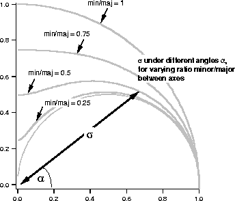
Note that distances from the point to the covariance ellipse do not describe the standard deviation along directions other than along the principal axes. This standard deviation is obtained by error propagation, and is greater than or equal to the distance to the error ellipse, the difference being explained by the non-uniform distribution of the second (angular) variable (see figure).

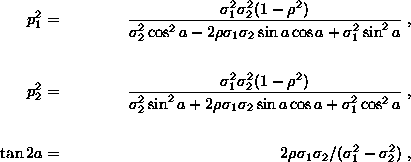
For vanishing correlation coefficient ( ) the principal axes of the error ellipse are parallel to the coordinate x₁, x₂ axes, and the principal semi-diameters of the ellipse p₁,p₂ are equal to .

For one can find the principal axes and their orientation with respect to the coordinate axes from the relations

where a is the angle between the x₁ axis and the semi-diameter of length p₁. Note that a is determined up to multiples of , i.e. for both semi-diameters of both principal axes.