Physics:PP/9/Comparing Data and Theory
| 99% complete | ||
|
|
Comparing Data and Theory
Comparing data and expectations (which can be a theory or some estimates using background-driven techniques) is not as simple as it may look at first [1]. In this section we will show several approaches used in particle physics, and illustrate how such approaches can be implemented in a real-life analysis code.
Ratio approach
If we have data and expectation (theory) histograms, the most popular approach is to show a ratio plot, i.e. divide each bin of a data histogram (D) by the the number of bin entries of a histogram "B" with an expectation (often called "background").
Let us show this using a ROOT file with two histograms, with the name "data" and "bkg" (from the word "background"). The background can be created using some theoretical computations. We will use the PPbook GitHub repository with the input data and auxiliary python modules. Let us download an example ROOT file and a small utility package that helps plotting data and theory histograms, as well as the ratio plots at the bottom of the main canvas.
wget https://raw.githubusercontent.com/chekanov/ppbook/master/histograms.root
wget https://raw.githubusercontent.com/chekanov/ppbook/master/utilpp.py
Now we will make a short pyROOT example code in which will read the two histograms, and divide them assuming that data and theory histograms are independent. The uncertainties will be propagated as discussed in Propagation of uncertainty section. Put these lines to "plot1.py", and run this file as "python plot1.py".
from utilpp import *
fr=TFile("histograms.root")
data, theory=fr.Get("data"), fr.Get("bkg")

def getRatio(data,theory):
  RAT=TGraphErrors()
  n=0
  for i in range(1,data.GetNbinsX()):
    D,B=data.GetBinContent(i),theory.GetBinContent(i)
    if (D>0 and B>0):
      x,ex=data.GetBinCenter(i),data.GetBinWidth(i)
      r1,r2 = data.GetBinError(i)/D, theory.GetBinError(i)/B
      y=D/B
      ey=y*math.sqrt(r1*r1 + r2*r2)
      RAT.SetPoint(n,x,y-1)
      RAT.SetPointError(n,ex,ey)
      n=n+1
  return RAT

X,Y,YR =[0,1E3,"X",0], [0.03,5E6,"Events",1], [-1.99,1.99,"Ratio",0]
showme("ppbook_c9_1.svg",data,theory,getRatio(data,theory),X,Y,YR)
In this example, we use the list [min,max,title,isLog] to define the axis.
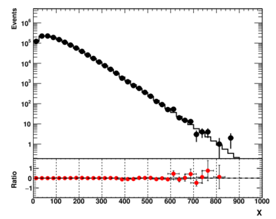
The output image of this script is
The data are shown as black symbols, while the theory expectation as the red line. The bottom plot shows their ratio.
Generally, this approach is very common for many practical cases. But, as corrected noted in [1], this is not a convenient way to compare two histograms when the bin contents span several orders of magnitude. In particle physics, exponentially decreasing distributions are extremely common due to the nature of the energy spectra. For example, exponentially decreasing distributions have energy spectra, transverse energy spectra, two-particle invariant masses etc. This "ratio" style representation shown above turns to hide significant discrepancies in the "bulk" of the distributions, where the density of entries are very large. To deal with this problem, one can calculate statistical significance.
Significance approach in Poisson approximation
For counting experiments with large numbers of entries per bin of a histogram, the Poisson distribution with the parameter "B" (representing the height of the histogram bin of expectations) can be approximated by a Gaussian with the mean "B" and the standard deviation [math]\displaystyle{ \sqrt{B} }[/math]. This leads to the following "Poisson" approximation for the z-value:
[math]\displaystyle{ z \simeq (D - B) / \sqrt{B} }[/math]
where "D" is the observed number of entries in the histogram bin. We can change the above Python code by replacing the ratio with this Poisson z-value.
from utilpp import *
fr=TFile("histograms.root")
data, theory =fr.Get("data"), fr.Get("bkg")

def getSign(data,theory):
  RAT=data.Clone()
  RAT.Reset()
  RAT.SetDirectory(0)
  for i in range(1,data.GetNbinsX()):
    D,B=data.GetBinContent(i),theory.GetBinContent(i)
    if (D>0 and B>0):
      y=(D-B)/math.sqrt(B)
      RAT.SetBinContent(i,y)
  return RAT

X, Y, YR =[0,1E3,"X",0], [0.03,5E6,"Events",1], [-6.99,6.99,"Sign.",0]
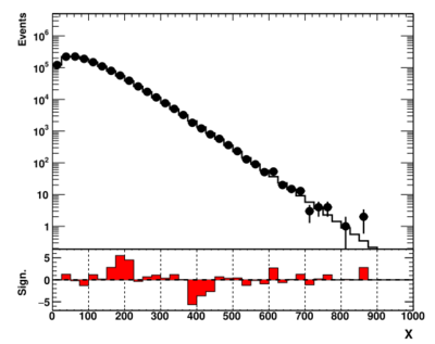
showme("ppbook_c9_2.svg",data,theory,getSign(data,theory),X,Y,YR)
This plot looks significantly better. Now we see two significant deviations from the expectation: an excess around 200 and a deficit around 400 (assuming arbitrary units).
Significance approach improved
The main disadvantage of the above approach is that, in low-population bins, the Poisson approximation is not a good approximation of the true z-values. Instead, we can plot the exact z-value in each bin. If a bin contains a significant excess of data (with p-value < 0.5), it will have a z-value > 0 which, when plotted, will give correctly the impression of an excess. The code shown below calculates the z-value without using the Poisson approximation:
from utilpp import *
fr=TFile("histograms.root")
data, theory =fr.Get("data"), fr.Get("bkg")

def getSig(data,theory):
  RAT=data.Clone()
  RAT.Reset()
  RAT.SetDirectory(0)
  for i in range(1,data.GetNbinsX()):
    D,B=data.GetBinContent(i),theory.GetBinContent(i)
    pVal=0
    if (B<=0): pVal=0.5
    if (D>B):  pVal=Math.inc_gamma(D,B)    # excess
    else:      pVal=Math.inc_gamma_c(D+1,B)
    zVal = GetZVal(pVal, D>B);
    if (pVal<0.5): RAT.SetBinContent(i, zVal)
  return RAT

X, Y, YR =[0,1E3,"X",0], [0.03,5E6,"Events",1], [-6.99,6.99,"Sign.",0]
showme("ppbook_c9_3.svg",data,theory,getSig(data,theory),X,Y,YR)
The definition of the function that transforms the p-value into the z-value can be found inside the "utilpp.py" module file.
Including theoretical uncertainties
When we show the ratio plot, we propagate the data and theory uncertainty assuming that the data and theory uncertainties are uncorrelated. However, it is more complicated to include the theory uncertainty into the significance value. It is obvious to expect that any additional uncertainty will decrease the significance of the observed deviations.
In the code shown below we will use the same approach as that discussed in [1]. Our p-value calculation will include the theory uncertainty which will be extracted from the theory histogram using GetBinError(i) method (returns a variance of expectations). Then we calculate the p-value for the Poisson distribution when there is uncertainty on the parameter "B". This is shown in the code below:
from utilpp import *
fr=TFile("histograms.root")
data,theory=fr.Get("data"),fr.Get("bkg")

def getSig(data,theory):
  RAT=data.Clone()
  RAT.Reset()
  RAT.SetDirectory(0)
  for i in range(1,data.GetNbinsX()):
    D,B=data.GetBinContent(i),theory.GetBinContent(i)
    if (D>0 and B>0):
       pVal = pValuePoissonError(D,B, theory.GetBinError(i))
       zVal = GetZVal(pVal, D>B)
       if (pVal<0.5): RAT.SetBinContent(i, zVal);
  return RAT

X,Y,YR = [0,1E3,"X",0], [0.03,5E6,"Events",1], [-6.99,6.99,"Sign.",0]
showme("ppbook_c9_4.svg",data,theory,getSig(data,theory),X,Y,YR)
The output is shown below:
This plot may look rather similar to the figure shown before, but the difference does exist. You can find the actual values by adding the "print(zVal)" statement in the last two code snippets. The statistical significance for the excesses is reduced by about 20% compared to the case when we assumed a theory without uncertainties.
Further details can be found in Ref. [1]. See also C++ implementation in [1]
References
- ↑ 1.0 1.1 1.2 1.3 Choudalakis, GeorgiosCasadei, Diego "Plotting the Differences Between Data and Expectation" Eur. Phys. J. Plus (2012) 127, p.25 arXiv: https://arxiv.org/abs/1111.2062


