Thin plate energy functional
The exact thin plate energy functional (TPEF) for a function [math]\displaystyle{ f(x,y) }[/math] is
- [math]\displaystyle{ \int_{y_0}^{y_1} \int_{x_0}^{x_1} (\kappa_1^2 + \kappa_2^2) \sqrt{g} \,dx \,dy }[/math]
where [math]\displaystyle{ \kappa_1 }[/math] and [math]\displaystyle{ \kappa_2 }[/math] are the principal curvatures of the surface mapping [math]\displaystyle{ f }[/math] at the point [math]\displaystyle{ (x,y). }[/math][1][2] This is the surface integral of [math]\displaystyle{ \kappa_1^2 + \kappa_2^2, }[/math] hence the [math]\displaystyle{ \sqrt{g} }[/math] in the integrand.
Minimizing the exact thin plate energy functional would result in a system of non-linear equations. So in practice, an approximation that results in linear systems of equations is often used.[1][3][4] The approximation is derived by assuming that the gradient of [math]\displaystyle{ f }[/math] is 0. At any point where [math]\displaystyle{ f_x = f_y =0, }[/math] the first fundamental form [math]\displaystyle{ g_{ij} }[/math] of the surface mapping [math]\displaystyle{ f }[/math] is the identity matrix and the second fundamental form [math]\displaystyle{ b_{ij} }[/math] is
- [math]\displaystyle{ \begin{pmatrix} f_{xx} & f_{xy} \\ f_{xy} & f_{yy} \end{pmatrix} }[/math].
We can use the formula for mean curvature [math]\displaystyle{ H=b_{ij}g^{ij}/2 }[/math][5] to determine that [math]\displaystyle{ H = (f_{xx}+f_{yy})/2 }[/math] and the formula for Gaussian curvature [math]\displaystyle{ K=b/g }[/math][5] (where [math]\displaystyle{ b }[/math] and [math]\displaystyle{ g }[/math] are the determinants of the second and first fundamental forms, respectively) to determine that [math]\displaystyle{ K=f_{xx}f_{yy} - (f_{xy})^2. }[/math] Since [math]\displaystyle{ H=(k_1+k_2)/2 }[/math] and [math]\displaystyle{ K=k_1k_2, }[/math][5] the integrand of the exact TPEF equals [math]\displaystyle{ 4H^2 - 2K. }[/math] The expressions we just computed for the mean curvature and Gaussian curvature as functions of partial derivatives of [math]\displaystyle{ f }[/math] show that the integrand of the exact TPEF is
- [math]\displaystyle{ 4H^2 - 2K = (f_{xx} + f_{yy})^2 - 2(f_{xx}f_{yy} - f_{xy}^2) = f_{xx}^2 + 2f_{xy}^2 + f_{yy}^2. }[/math]
So the approximate thin plate energy functional is
- [math]\displaystyle{ J[f] = \int_{y_0}^{y_1} \int_{x_0}^{x_1} f_{xx}^2 + 2f_{xy}^2 + f_{yy}^2 \,dx \,dy. }[/math]
Rotational invariance
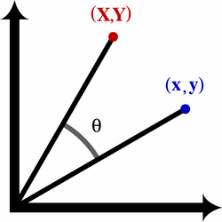
The TPEF is rotationally invariant. This means that if all the points of the surface [math]\displaystyle{ z(x,y) }[/math] are rotated by an angle [math]\displaystyle{ \theta }[/math] about the [math]\displaystyle{ z }[/math]-axis, the TPEF at each point [math]\displaystyle{ (x,y) }[/math] of the surface equals the TPEF of the rotated surface at the rotated [math]\displaystyle{ (x,y). }[/math] The formula for a rotation by an angle [math]\displaystyle{ \theta }[/math] about the [math]\displaystyle{ z }[/math]-axis is
-
[math]\displaystyle{ \binom{X}{Y} = \begin{pmatrix} \cos\theta & -\sin\theta \\ \sin\theta & \cos\theta \end{pmatrix}\binom{x}{y} = R\binom{x}{y}. }[/math]
()
The fact that the [math]\displaystyle{ z }[/math] value of the surface at [math]\displaystyle{ (x,y) }[/math] equals the [math]\displaystyle{ z }[/math] value of the rotated surface at the rotated [math]\displaystyle{ (x,y) }[/math] is expressed mathematically by the equation
- [math]\displaystyle{ Z(X,Y) = z(x,y) = (z\circ xy)(X,Y) }[/math]
where [math]\displaystyle{ xy }[/math] is the inverse rotation, that is, [math]\displaystyle{ xy(X,Y) = R^{-1}(X, Y)^{\text{T}} = R^{\text{T}}(X,Y)^{\text{T}}. }[/math] So [math]\displaystyle{ Z = z\circ xy }[/math] and the chain rule implies
-
[math]\displaystyle{ Z_i = z_j R_{ij}. }[/math]
()
In equation (2), [math]\displaystyle{ Z_0 }[/math] means [math]\displaystyle{ Z_X, }[/math] [math]\displaystyle{ Z_1 }[/math] means [math]\displaystyle{ Z_Y, }[/math] [math]\displaystyle{ z_0 }[/math] means [math]\displaystyle{ z_x, }[/math] and [math]\displaystyle{ z_1 }[/math] means [math]\displaystyle{ z_y. }[/math] Equation (2) and all subsequent equations in this section use non-tensor summation convention, that is, sums are taken over repeated indices in a term even if both indices are subscripts. The chain rule is also needed to differentiate equation (2) since [math]\displaystyle{ z_j }[/math] is actually the composition [math]\displaystyle{ z_j \circ xy: }[/math]
- [math]\displaystyle{ Z_{ik} = z_{jl}R_{kl} R_{ij} }[/math].
Swapping the index names [math]\displaystyle{ j }[/math] and [math]\displaystyle{ k }[/math] yields
-
[math]\displaystyle{ Z_{ij} = z_{kl}R_{jl}R_{ik}. }[/math]
()
Expanding the sum for each pair [math]\displaystyle{ i,j }[/math] yields
- [math]\displaystyle{ \begin{array}{lcl} Z_{XX} & = & R_{00}^2 z_{xx} + 2R_{00}R_{01}z_{xy} + R_{01}^2 z_{yy}, \\ Z_{XY} & = & R_{00}R_{10}z_{xx} + (R_{00}R_{11} + R_{01}R_{10})z_{xy} + R_{01}R_{11}z_{yy}, \\ Z_{YY} & = & R_{10}^2 z_{xx} + 2R_{10}R_{11}z_{xy} + R_{11}^2 z_{yy}. \end{array} }[/math]
Computing the TPEF for the rotated surface yields
-
[math]\displaystyle{ \begin{align} Z_{XX}^2 + 2 Z_{XY}^2 + Z_{YY}^2 &= (R_{11}^2 + R_{01}^2) z_{yy}^2 \\ &+ 2(R_{10}R_{11} + R_{00}R_{01})^2 z_{xx} z_{yy} \\ &+ 2(2R_{10}^2R_{11}^2 + R_{00}^2R_{11}^2 + 2R_{00}R_{01}R_{10}R_{11} \\ &\qquad + R_{01}^2R_{10}^2 + 2R_{00}^2R_{01}^2)z_{xy}^2 \\ &+ 4(R_{10}R_{11} + R_{00}R_{01})(R_{11}^2 + R_{01}^2) z_{xy}z_{yy} \\ &+ 4(R_{10}^2 + R_{00}^2)(R_{10}R_{11} + R_{00}R_{01}) z_{xx}z_{xy} \\ &+ (R_{10}^2 + R_{00}^2)z_{xx}^2. \\ \end{align} }[/math]
()
Inserting the coefficients of the rotation matrix [math]\displaystyle{ R }[/math] from equation (1) into the right-hand side of equation (4) simplifies it to [math]\displaystyle{ z_{xx}^2 + 2 z_{xy}^2 + z_{yy}^2. }[/math]
Data fitting
The approximate thin plate energy functional can be used to fit B-spline surfaces to scattered 1D data on a 2D grid (for example, digital terrain model data).[6][3] Call the grid points [math]\displaystyle{ (x_i,y_i) }[/math] for [math]\displaystyle{ i=1\dots N }[/math] (with [math]\displaystyle{ x_i \in [a,b] }[/math] and [math]\displaystyle{ y_i \in [c,d] }[/math]) and the data values [math]\displaystyle{ z_i. }[/math] In order to fit a uniform B-spline [math]\displaystyle{ f(x,y) }[/math] to the data, the equation
-
[math]\displaystyle{ \sum_{i=1}^N (f(x_i,y_i) - z_i)^2 + \lambda \int_{c}^{d} \int_{a}^{b} (f_{xx}^2 + 2f_{xy}^2 + f_{yy}^2) \,dx \,dy }[/math]
()
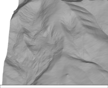
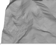
(where [math]\displaystyle{ \lambda }[/math] is the "smoothing parameter") is minimized. Larger values of [math]\displaystyle{ \lambda }[/math] result in a smoother surface and smaller values result in a more accurate fit to the data. The following images illustrate the results of fitting a B-spline surface to some terrain data using this method.
The thin plate smoothing spline also minimizes equation (5), but it is much more expensive to compute than a B-spline and not as smooth (it is only [math]\displaystyle{ C^1 }[/math] at the "centers" and has unbounded second derivatives there).
References
- ↑ 1.0 1.1 Greiner, Günther (1994). "Variational Design and Fairing of Spline Surfaces". Eurographics '94. http://mrl.nyu.edu/~elif/thesisprop/Greiner94.pdf?origin=publication_detail. Retrieved January 3, 2016.
- ↑ Moreton, Henry P. (1992). "Functional Optimization for Fair Surface Design". Computer Graphics. http://www.cs.berkeley.edu/~sequin/PAPERS/SIGGR92_MVC_MVS.pdf. Retrieved January 4, 2016.
- ↑ 3.0 3.1 Eck, Matthias (1996). "Automatic reconstruction of B-splines surfaces of arbitrary topological type". Proceedings of SIGGRAPH 96, Computer Graphics Proceedings, Annual Conference Series. http://www.cs.hunter.cuny.edu/~ioannis/3DP_F03/PAPERS/MODELING/HOPPE/bspline.pdf. Retrieved January 3, 2016.
- ↑ Halstead, Mark (1993). "Efficient, Fair Interpolation using Catmull-Clark Surfaces". Proceedings of the 20th annual conference on Computer graphics and interactive techniques. http://graphics.pixar.com/people/derose/publications/FairSubdivision/paper.pdf. Retrieved January 4, 2016.
- ↑ 5.0 5.1 5.2 Kreyszig, Erwin (1991). Differential Geometry. Mineola, New York: Dover. pp. 131. ISBN 0-486-66721-9. https://archive.org/details/differentialgeom00krey.
- ↑ Hjelle, Oyvind (2005). "Multilevel Least Squares Approximation of Scattered Data over Binary Triangulations". Computing and Visualization in Science. http://home.simula.no/~oyvindhj/pub/lsbintrSpringer.pdf. Retrieved January 14, 2016.
 |


