Method of averaging
In mathematics, more specifically in dynamical systems, the method of averaging (also called averaging theory) exploits systems containing time-scales separation: a fast oscillation versus a slow drift. It suggests that we perform an averaging over a given amount of time in order to iron out the fast oscillations and observe the qualitative behavior from the resulting dynamics. The approximated solution holds under finite time inversely proportional to the parameter denoting the slow time scale. It turns out to be a customary problem where there exists the trade off between how good is the approximated solution balanced by how much time it holds to be close to the original solution.
More precisely, the system has the following form [math]\displaystyle{ \dot{x} = \varepsilon f( x,t , \varepsilon ), \quad 0 \leq \varepsilon \ll 1 }[/math]of a phase space variable [math]\displaystyle{ x. }[/math]The fast oscillation is given by [math]\displaystyle{ f }[/math] versus a slow drift of [math]\displaystyle{ \dot{x} }[/math]. The averaging method yields an autonomous dynamical system [math]\displaystyle{ \dot{y}= \varepsilon {\frac {1}{T}}\int _{0}^{T}f(y, s, 0)~ds =: \varepsilon {\bar {f}}(y) }[/math] which approximates the solution curves of [math]\displaystyle{ \dot{x} }[/math] inside a connected and compact region of the phase space and over time of [math]\displaystyle{ 1/\varepsilon }[/math].
Under the validity of this averaging technique, the asymptotic behavior of the original system is captured by the dynamical equation for [math]\displaystyle{ y }[/math]. In this way, qualitative methods for autonomous dynamical systems may be employed to analyze the equilibria and more complex structures, such as slow manifold and invariant manifolds, as well as their stability in the phase space of the averaged system.
In addition, in a physical application it might be reasonable or natural to replace a mathematical model, which is given in the form of the differential equation for [math]\displaystyle{ \dot{x} }[/math], with the corresponding averaged system [math]\displaystyle{ \dot{y} }[/math], in order to use the averaged system to make a prediction and then test the prediction against the results of a physical experiment.[1]
The averaging method has a long history, which is deeply rooted in perturbation problems that arose in celestial mechanics (see, for example in [2]).
First example

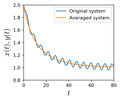
Consider a perturbed logistic growth [math]\displaystyle{ \dot {x} = \varepsilon (x (1 - x) + \sin{t}) \quad \quad x \in \R, \quad 0 \leq \varepsilon \ll 1, }[/math] and the averaged equation [math]\displaystyle{ \dot {y} = \varepsilon y (1 - y) \qquad y \in \R. }[/math]The purpose of the method of averaging is to tell us the qualitative behavior of the vector field when we average it over a period of time. It guarantees that the solution [math]\displaystyle{ y(t) }[/math] approximates [math]\displaystyle{ x(t) }[/math] for times [math]\displaystyle{ t = \mathcal{O}(1/\varepsilon). }[/math] Exceptionally: in this example the approximation is even better, it is valid for all times. We present it in a section below.
Definitions
We assume the vector field [math]\displaystyle{ f:\R^n \times \R \times \R \to \R^n }[/math] to be of differentiability class [math]\displaystyle{ C^{r} }[/math] with [math]\displaystyle{ r \geq 2 }[/math] (or even we will only say smooth), which we will denote [math]\displaystyle{ f \in C^r(\R^n \times \R \times \R^+; \R^n) }[/math]. We expand this time-dependent vector field in a Taylor series (in powers of [math]\displaystyle{ \varepsilon }[/math]) with remainder [math]\displaystyle{ f^{[k + 1]}(x, t, \varepsilon) }[/math]. We introduce the following notation:[2] [math]\displaystyle{ f(x, t, \varepsilon) = f^0(x, t) + \varepsilon f^{1}(x, t) + \dots + \varepsilon^k f^{k}(x, t) + \varepsilon^{k + 1} f^{[k + 1]}(x, t, \varepsilon), }[/math] where [math]\displaystyle{ f^{j} = \frac{f^{(j)}(x, t, 0)}{j!} }[/math]is the [math]\displaystyle{ j }[/math]-th derivative with [math]\displaystyle{ 0 \leq j \leq k }[/math]. As we are concerned with averaging problems, in general [math]\displaystyle{ f^0(x, t) }[/math] is zero, so it turns out that we will be interested in vector fields given by [math]\displaystyle{ f(x, t, \varepsilon) = \varepsilon f^{[1]}(x, t, \varepsilon) = \varepsilon f^{1}(x, t) + \varepsilon^{2} f^{[2]}(x, t, \varepsilon). }[/math] Besides, we define the following initial value problem to be in the standard form:[2] [math]\displaystyle{ \dot{x} = \varepsilon f^{1}(x, t) + \varepsilon^{2} f^{[2]}(x, t, \varepsilon), \qquad x(0, \varepsilon) =: x_0 \in D \subseteq \R^n, \quad 0 \leq \varepsilon \ll 1. }[/math]
Theorem: averaging in the periodic case
Consider for every [math]\displaystyle{ D \subset \R^n }[/math] connected and bounded and every [math]\displaystyle{ \varepsilon_0 \gt 0 }[/math] there exist [math]\displaystyle{ L \gt 0 }[/math] and [math]\displaystyle{ \varepsilon \leq \varepsilon_0 }[/math] such that the original system (a non-autonomous dynamical system) given by [math]\displaystyle{ \dot{x} = \varepsilon f^{1}(x, t) + \varepsilon^{2} f^{[2]}(x, t, \varepsilon), \qquad x_0 \in D \subseteq \R^n, \quad 0 \leq \varepsilon \ll 1, }[/math] has solution [math]\displaystyle{ x(t, \varepsilon) }[/math], where [math]\displaystyle{ f^1 \in C^r(D \times \R; \R^n) }[/math] is periodic with period [math]\displaystyle{ T }[/math] and [math]\displaystyle{ f^{[2]} \in C^r(D \times \R \times \R^+; \R^n) }[/math] both with [math]\displaystyle{ r \geq 2 }[/math] bounded on bounded sets. Then there exists a constant [math]\displaystyle{ c \gt 0 }[/math] such that the solution [math]\displaystyle{ y(t, \varepsilon) }[/math] of the averaged system (autonomous dynamical system) is [math]\displaystyle{ \dot{y}= \varepsilon {\frac {1}{T}} \int _{0}^{T}f^1(y, s)~ds =: \varepsilon{\bar {f}}^1(y), \quad y(0, \varepsilon) = x_0 }[/math] is [math]\displaystyle{ \|x(t, \varepsilon) - y(t, \varepsilon)\| \lt c \varepsilon }[/math]for [math]\displaystyle{ 0 \leq \varepsilon \leq \varepsilon_0 }[/math] and [math]\displaystyle{ 0 \leq t \leq L/\varepsilon }[/math].
Remarks
- There are two approximations in this what is called first approximation estimate: reduction to the average of the vector field and negligence of [math]\displaystyle{ \mathcal{O}(\varepsilon^2) }[/math] terms.
- Uniformity with respect to the initial condition [math]\displaystyle{ x_0 }[/math]: if we vary [math]\displaystyle{ x_0 }[/math] this affects the estimation of [math]\displaystyle{ L }[/math] and [math]\displaystyle{ c }[/math]. The proof and discussion of this can be found in J. Murdock's book.[3]
- Reduction of regularity: there is a more general form of this theorem which requires only [math]\displaystyle{ f^1 }[/math] to be Lipschitz and [math]\displaystyle{ f^{[2]} }[/math] continuous. It is a more recent proof and can be seen in Sanders et al..[2] The theorem statement presented here is due to the proof framework proposed by Krylov-Bogoliubov which is based on an introduction of a near-identity transformation. The advantage of this method is the extension to more general settings such as infinite-dimensional systems - partial differential equation or delay differential equations.
- J. Hale presents generalizations to almost periodic vector-fields.[4]
Strategy of the proof
Krylov-Bogoliubov realized that the slow dynamics of the system determines the leading order of the asymptotic solution.
In order to proof it, they proposed a near-identity transformation, which turned out to be a change of coordinates with its own time-scale transforming the original system to the averaged one.
Sketch of the proof
- Determination of a near-identity transformation: the smooth mapping [math]\displaystyle{ y \mapsto U(y, t, \varepsilon) = y + \varepsilon u^{[1]}(y, t, \varepsilon) }[/math]where [math]\displaystyle{ u^{[1]} }[/math] is assumed to be regular enough and [math]\displaystyle{ T }[/math] periodic. The proposed change of coordinates is given by [math]\displaystyle{ x = U(y, t, \varepsilon) }[/math].
- Choose an appropriate [math]\displaystyle{ u^{[1]} }[/math]solving the homological equation of the averaging theory: [math]\displaystyle{ \frac{\partial u^{[1]}}{\partial t} = f^{1}(y, t) - \bar{f}^1(y) }[/math].
- Change of coordinates carries the original system to [math]\displaystyle{ \dot{y} = \varepsilon \bar{f}^1(y) + \varepsilon^2 f_{*}^{[2]}(y, t, \varepsilon). }[/math]
- Estimation of error due to truncation and comparison to the original variable.
Non-autonomous class of systems: more examples
Along the history of the averaging technique, there is class of system extensively studied which give us meaningful examples we will discuss below. The class of system is given by: [math]\displaystyle{ \ddot{z} + z = \varepsilon g(z, \dot{z}, t), \qquad z \in \R,\quad z(0) = z_0 ~\mathrm{ and }~ \dot{z}(0) = v_0, }[/math] where [math]\displaystyle{ g }[/math] is smooth. This system is similar to a linear system with a small nonlinear perturbation given by [math]\displaystyle{ \begin{bmatrix} 0 \\ \varepsilon ~g(z, \dot{z}, t) \end{bmatrix} }[/math]: [math]\displaystyle{ \begin{aligned} \dot{z_1} &= z_2, & z_1(0) &= z_0 \\ \dot{z_2} &= -z_1 + \varepsilon g(z_1, z_2, t), & z_2(0) &= v_0, \end{aligned} }[/math] differing from the standard form. Hence there is a necessity to perform a transformation to make it in the standard form explicitly.[2] We are able to change coordinates using variation of constants method. We look at the unperturbed system, i.e. [math]\displaystyle{ \varepsilon = 0 }[/math], given by [math]\displaystyle{ \begin{bmatrix} \dot{z_1} \\ \dot{z_2} \end{bmatrix} = \begin{bmatrix} 0 & 1 \\ -1 & 0 \end{bmatrix} \begin{bmatrix} z_1 \\ z_2 \end{bmatrix} = A \begin{bmatrix} z_1 \\ z_2 \end{bmatrix} }[/math]
which has the fundamental solution [math]\displaystyle{ \Phi(t) = e^{A t} }[/math]corresponding to a rotation. Then the time-dependent change of coordinates is [math]\displaystyle{ z(t) = \Phi(t) x }[/math] where [math]\displaystyle{ x }[/math] is the coordinates respective to the standard form.
If we take the time derivative in both sides and invert the fundamental matrix we obtain [math]\displaystyle{ \dot{x} = \varepsilon e^{- A t} \begin{bmatrix} 0 \\ ~\tilde g(x, \dot{x}, t) \end{bmatrix} ~\text{ with }~ \tilde g(x, \dot{x}, t)=g(\cos(t)x(t)+\sin(t)\dot x(t), -\sin(t)x(t)+\cos(t)\dot x(t), t). }[/math]
Remarks
- The same can be done to time-dependent linear parts. Although the fundamental solution may be non-trivial to write down explicitly, the procedure is similar. See Sanders et al. [2] for further details.
- If the eigenvalues of [math]\displaystyle{ A }[/math] are not all purely imaginary this is called hyperbolicity condition. For this occasion, the perturbation equation may present some serious problems even whether [math]\displaystyle{ g }[/math] is bounded, since the solution grows exponentially fast.[2] However, qualitatively, we may be able to know the asymptotic solution, such as Hartman-Grobman results and more.[1]
- Occasionally, polar coordinates may yield standard forms that are simpler to analyze. Consider [math]\displaystyle{ z_1 = r \sin(t - \phi) ~\text{and}~ z_2 = r \cos(t - \phi) }[/math], which determines the initial condition [math]\displaystyle{ (r(0), \phi(0)) }[/math] and the system [math]\displaystyle{ \begin{bmatrix} \dot{r} \\ \dot{\phi} \end{bmatrix} = \varepsilon \begin{bmatrix} \cos(t - \phi) g(r \sin(t - \phi), r \cos(t - \phi), t) \\ \frac{1}{r} \sin(t - \phi) g(r \sin(t - \phi), r \cos(t - \phi), t) \end{bmatrix}. }[/math]
If [math]\displaystyle{ g \in C^1 }[/math]we may apply averaging so long as a neighborhood of the origin is excluded (since the polar coordinates fail): [math]\displaystyle{ \begin{array}{rcl} \bar{f}_1^1(r) & = & \displaystyle \frac{1}{2 \pi} \int_0^{2 \pi} \cos(s - \phi) g(r \sin (s - \phi), r \cos(s - \phi), s) ds \\[4pt] \bar{f}_2^1(r) & = & \displaystyle \frac{1}{2 \pi r} \int_0^{2 \pi} \sin(s - \phi) g(r \sin (s - \phi), r \cos(s - \phi), s) ds, \end{array} }[/math] where the averaged system is [math]\displaystyle{ \begin{array}{lcr} \dot{\bar{r}} = \varepsilon \bar{f}_1^1 (\bar{r}) \\ \dot{\bar{\phi}} = \varepsilon \bar{f}_2^1 (\bar{r}). \end{array} }[/math]
Example: Misleading averaging results

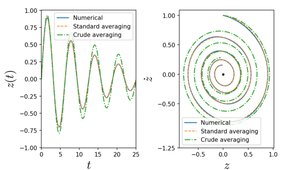
The method contains some assumptions and restrictions. These limitations play important role when we average the original equation which is not into the standard form, and we can discuss counterexample of it. The following example in order to discourage this hurried averaging:[2] [math]\displaystyle{ \ddot{z} + 4 \varepsilon \cos^2{(t)} \dot{z} + z = 0, \qquad z(0) = 0,\quad \dot{z}(0) = 1, }[/math]where we put [math]\displaystyle{ g(z, \dot{z}, t) = - 4\cos^2(t) \dot{z} }[/math]following the previous notation.
This systems corresponds to a damped harmonic oscillator where the damping term oscillates between [math]\displaystyle{ 0 }[/math] and [math]\displaystyle{ 4\varepsilon }[/math]. Averaging the friction term over one cycle of [math]\displaystyle{ 2 \pi }[/math] yields the equation: [math]\displaystyle{ \ddot{\bar{z}} + 2 \varepsilon \dot{\bar{z}} + \bar{z} = 0, \qquad \bar{z}(0) = 0, \quad \dot{\bar{z}}(0) = 1. }[/math]The solution is [math]\displaystyle{ \bar{z}(t) = \frac{1}{(1 - \varepsilon^2)^{\frac{1}{2}}} e^{- \varepsilon t} \sin{((1 - \varepsilon^2)^{\frac{1}{2}}t)}. }[/math] which the convergence rate to the origin is [math]\displaystyle{ \varepsilon }[/math]. The averaged system obtained from the standard form yields: [math]\displaystyle{ \begin{array}{lcr} \dot{\bar{r}} = - \frac{1}{2}\varepsilon \bar{r}(2 + \cos(2 \bar{\phi})), ~\bar{r}(0) = 1 \\ \dot{\bar{\phi}} = \frac{1}{2}\varepsilon \sin(2 \bar{\phi}), ~\bar{\phi}(0) = 0, \end{array} }[/math] which in the rectangular coordinate shows explicitly that indeed the rate of convergence to the origin is [math]\displaystyle{ \frac{3}{2} \varepsilon }[/math] differing from the previous crude averaged system: [math]\displaystyle{ y(t) = e^{-\frac{3}{2} \varepsilon t} \sin{t} }[/math]
Example: Van der Pol Equation

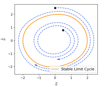
Van der Pol was concerned with obtaining approximate solutions for equations of the type [math]\displaystyle{ \ddot{z} + \varepsilon (1 - z^2) \dot{z} + z = 0, }[/math] where [math]\displaystyle{ g(z, \dot{z}, t) = (1 - z^2) \dot{z} }[/math] following the previous notation. This system is often called the Van der Pol oscillator. Applying periodic averaging to this nonlinear oscillator provides qualitative knowledge of the phase space without solving the system explicitly.
The averaged system is [math]\displaystyle{ \begin{array}{lcr} \dot{\bar{r}} = \frac{1}{2}\varepsilon \bar{r}(1 - \frac{1}{4} \bar{r}^2) \\ \dot{\bar{\phi}} = 0, \end{array} }[/math] and we can analyze the fixed points and their stability. There is an unstable fixed point at the origin and a stable limit cycle represented by [math]\displaystyle{ \bar{r} = 2 }[/math].
The existence of such stable limit-cycle can be stated as a theorem.
Theorem (Existence of a periodic orbit)[5]: If [math]\displaystyle{ p_0 }[/math]is a hyperbolic fixed point of
[math]\displaystyle{ \dot{y}= \varepsilon {\bar {f}}^1(y) }[/math]Then there exists [math]\displaystyle{ \varepsilon_0 \gt 0 }[/math]such that for all [math]\displaystyle{ 0 \lt \varepsilon \lt \varepsilon_0 }[/math],
[math]\displaystyle{ \dot{x} = \varepsilon f^{1}(x, t) + \varepsilon^{2} f^{[2]}(x, t, \varepsilon) }[/math]
has a unique hyperbolic periodic orbit [math]\displaystyle{ \gamma_{\varepsilon}(t) = p_0 + \mathcal{O}(\varepsilon) }[/math] of the same stability type as [math]\displaystyle{ p_0 }[/math].
The proof can be found at Guckenheimer and Holmes,[5] Sanders et al. [2] and for the angle case in Chicone.[1]
Example: Restricting the time interval

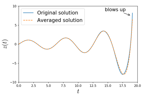
The average theorem assumes existence of a connected and bounded region [math]\displaystyle{ D \subset \R^n }[/math]which affects the time interval [math]\displaystyle{ L }[/math] of the result validity. The following example points it out. Consider the [math]\displaystyle{ \ddot{z} + z = 8 \varepsilon \cos{(t)} \dot{z}^2 , ~ z(0) = 0,~ \dot{z}(0) = 1, }[/math] where [math]\displaystyle{ g(z, \dot{z}, t) = 8 \dot{z}^2 \cos(t) }[/math]. The averaged system consists of [math]\displaystyle{ \begin{array}{lcr} \dot{\bar{r}} = 3 \varepsilon \bar{r}^2\cos(\bar{\phi}), ~\bar{r}(0) = 1 \\ \dot{\bar{\phi}} = -\varepsilon \bar{r} \sin(\bar{\phi}), ~\bar{\phi}(0) = 0, \end{array} }[/math] which under this initial condition indicates that the original solution behaves like [math]\displaystyle{ z(t) = \frac{\sin(t)}{1 - 3 \varepsilon t} + \mathcal{O}(\varepsilon), }[/math] where it holds on a bounded region over [math]\displaystyle{ 0 \leq \varepsilon t \leq L \lt \frac{1}{3} }[/math].
Damped Pendulum
Consider a damped pendulum whose point of suspension is vibrated vertically by a small amplitude, high frequency signal (this is usually known as dithering). The equation of motion for such a pendulum is given by [math]\displaystyle{ m(l\ddot{\theta} - ak\omega^2 \sin \omega t \sin \theta) = -mg \sin \theta - k(l\dot{\theta} + a\omega \cos \omega t \sin \theta) }[/math] where [math]\displaystyle{ a \sin \omega t }[/math] describes the motion of the suspension point, [math]\displaystyle{ k }[/math] describes the damping of the pendulum, and [math]\displaystyle{ \theta }[/math] is the angle made by the pendulum with the vertical.
The phase space form of this equation is given by [math]\displaystyle{ \begin{align} \dot t &= 1 \\ \dot\theta &= p \\ \dot p &= \frac{1}{ml} (mak\omega^2 \sin\omega t \sin \theta - mg\sin\theta - k(l p + a\omega \cos\omega t \sin \theta)) \end{align} }[/math] where we have introduced the variable [math]\displaystyle{ p }[/math] and written the system as an autonomous, first-order system in [math]\displaystyle{ (t, \theta, p) }[/math]-space.
Suppose that the angular frequency of the vertical vibrations, [math]\displaystyle{ \omega }[/math], is much greater than the natural frequency of the pendulum, [math]\displaystyle{ \sqrt{ g/l } }[/math]. Suppose also that the amplitude of the vertical vibrations, [math]\displaystyle{ a }[/math], is much less than the length [math]\displaystyle{ l }[/math] of the pendulum. The pendulum's trajectory in phase space will trace out a spiral around a curve [math]\displaystyle{ C }[/math], moving along [math]\displaystyle{ C }[/math] at the slow rate [math]\displaystyle{ \sqrt{ g/l } }[/math] but moving around it at the fast rate [math]\displaystyle{ \omega }[/math]. The radius of the spiral around [math]\displaystyle{ C }[/math] will be small and proportional to [math]\displaystyle{ a }[/math]. The average behaviour of the trajectory, over a timescale much larger than [math]\displaystyle{ 2\pi/\omega }[/math], will be to follow the curve [math]\displaystyle{ C }[/math].
Extension error estimates
Average technique for initial value problems has been treated up to now with an validity error estimates of order [math]\displaystyle{ 1/\varepsilon }[/math]. However, there are circumstances where the estimates can be extended for further times, even the case for all times.[2] Below we deal with a system containing an asymptotically stable fixed point. Such situation recapitulates what is illustrated in Figure 1.
Theorem (Eckhaus [6]/Sanchez-Palencia [7]) Consider the initial value problem [math]\displaystyle{ \dot{x} = \varepsilon f^{1}(x, t), \qquad x_0 \in D \subseteq \R^n, \quad 0 \leq \varepsilon \ll 1. }[/math] Suppose [math]\displaystyle{ \dot{y}= \varepsilon \lim_{T \to \infty}{\frac {1}{T}}\int _{0}^{T}f^1(y, s)~ds =: \varepsilon{\bar {f}}^1(y), \quad y(0, \varepsilon) = x_0 }[/math] exists and contains an asymptotically stable fixed point [math]\displaystyle{ y = 0 }[/math] in the linear approximation. Moreover, [math]\displaystyle{ \bar{f}^1 }[/math]is continuously differentiable with respect to [math]\displaystyle{ y }[/math] in [math]\displaystyle{ D }[/math] and has a domain of attraction [math]\displaystyle{ D^0 \subset D }[/math]. For any compact [math]\displaystyle{ K \subset D^0 }[/math] and for all [math]\displaystyle{ x_0 \in K }[/math] [math]\displaystyle{ \|x(t) - y(t)\| = \mathcal{O}(\delta(\varepsilon)), \quad 0 \leq t \lt \infty, }[/math] with [math]\displaystyle{ \delta(\varepsilon) = o(1) }[/math] in the general case and [math]\displaystyle{ \mathcal{O}(\varepsilon) }[/math] in the periodic case.
References
- ↑ 1.0 1.1 1.2 Charles., Chicone, Carmen (2006). Ordinary differential equations with applications (2nd ed.). New York: Springer. ISBN 9780387307695. OCLC 288193020.
- ↑ 2.0 2.1 2.2 2.3 2.4 2.5 2.6 2.7 2.8 2.9 Sanders, Jan A.; Verhulst, Ferdinand; Murdock, James (2007) (in en-gb). Averaging Methods in Nonlinear Dynamical Systems. Applied Mathematical Sciences. 59. doi:10.1007/978-0-387-48918-6. ISBN 978-0-387-48916-2.
- ↑ Murdock, James A. (1999). Perturbations : theory and methods. Philadelphia: Society for Industrial and Applied Mathematics. ISBN 978-0898714432. OCLC 41612407.
- ↑ Hale, Jack K. (1980). Ordinary differential equations (2nd ed.). Huntington, N.Y.: R.E. Krieger Pub. Co. ISBN 978-0898740110. OCLC 5170595.
- ↑ 5.0 5.1 Guckenheimer, John; Holmes, Philip (1983) (in en-gb). Nonlinear Oscillations, Dynamical Systems, and Bifurcations of Vector Fields. Applied Mathematical Sciences. 42. doi:10.1007/978-1-4612-1140-2. ISBN 978-1-4612-7020-1.
- ↑ Eckhaus, Wiktor (1975-03-01). "New approach to the asymptotic theory of nonlinear oscillations and wave-propagation". Journal of Mathematical Analysis and Applications 49 (3): 575–611. doi:10.1016/0022-247X(75)90200-0. ISSN 0022-247X.
- ↑ Sanchez-Palencia, Enrique (1976-01-01). "Methode de centrage-estimation de l'erreur et comportement des trajectoires dans l'espace des phases". International Journal of Non-Linear Mechanics 11 (4): 251–263. doi:10.1016/0020-7462(76)90004-4. ISSN 0020-7462. Bibcode: 1976IJNLM..11..251S.
 |

