Ranking SVM

Short description: Variant of the SVM algorithm

In machine learning, a ranking SVM is a variant of the support vector machine algorithm, which is used to solve certain ranking problems (via learning to rank). The ranking SVM algorithm was published by Thorsten Joachims in 2002. The original purpose of the algorithm was to improve the performance of an internet search engine. However, it was found that ranking SVM also can be used to solve other problems such as Rank SIFT.

Description

The ranking SVM algorithm is a learning retrieval function that employs pairwise ranking methods to adaptively sort results based on how 'relevant' they are for a specific query. The ranking SVM function uses a mapping function to describe the match between a search query and the features of each of the possible results. This mapping function projects each data pair (such as a search query and clicked web-page, for example) onto a feature space. These features are combined with the corresponding click-through data (which can act as a proxy for how relevant a page is for a specific query) and can then be used as the training data for the ranking SVM algorithm.

Generally, ranking SVM includes three steps in the training period:

1. It maps the similarities between queries and the clicked pages onto a certain feature space.
2. It calculates the distances between any two of the vectors obtained in step 1.
3. It forms an optimization problem which is similar to a standard SVM classification and solves this problem with the regular SVM solver.

Background

Ranking method

Suppose [math]\displaystyle{ \mathbb{C} }[/math] is a data set containing [math]\displaystyle{ N }[/math] elements [math]\displaystyle{ c_i }[/math]. [math]\displaystyle{ r }[/math] is a ranking method applied to [math]\displaystyle{ \mathbb{C} }[/math]. Then the [math]\displaystyle{ r }[/math] in [math]\displaystyle{ \mathbb{C} }[/math] can be represented as a [math]\displaystyle{ N \times N }[/math] binary matrix. If the rank of [math]\displaystyle{ c_i }[/math] is higher than the rank of [math]\displaystyle{ c_j }[/math], i.e. [math]\displaystyle{ r\ c_i \lt r\ c_j }[/math], the corresponding position of this matrix is set to value of "1". Otherwise the element in that position will be set as the value "0".

Kendall's tau

Kendall's Tau also refers to Kendall tau rank correlation coefficient, which is commonly used to compare two ranking methods for the same data set.

Suppose [math]\displaystyle{ r_1 }[/math] and [math]\displaystyle{ r_2 }[/math] are two ranking method applied to data set [math]\displaystyle{ \mathbb{C} }[/math], the Kendall's Tau between [math]\displaystyle{ r_1 }[/math] and [math]\displaystyle{ r_2 }[/math] can be represented as follows:

[math]\displaystyle{ \tau (r_1,r_2) = {P-Q \over P+Q} = 1- {2Q \over P+Q} }[/math]

where [math]\displaystyle{ P }[/math] is the number of concordant pairs and [math]\displaystyle{ Q }[/math] is the number of discordant pairs (inversions). A pair [math]\displaystyle{ d_i }[/math] and [math]\displaystyle{ d_j }[/math] is concordant if both [math]\displaystyle{ r_a }[/math] and [math]\displaystyle{ r_b }[/math] agree in how they order [math]\displaystyle{ d_i }[/math] and [math]\displaystyle{ d_j }[/math] . It is discordant if they disagree.

Information retrieval quality

Information retrieval quality is usually evaluated by the following three measurements:

1. Precision
2. Recall
3. Average precision

For a specific query to a database, let [math]\displaystyle{ P_{relevant} }[/math] be the set of relevant information elements in the database and [math]\displaystyle{ P_{retrieved} }[/math] be the set of the retrieved information elements. Then the above three measurements can be represented as follows:

[math]\displaystyle{ \begin{align} & \text{precision} = \frac{ \left| P_\text{relevant} \cap P_\text{retrieved} \right|}{\left| P_\text{retrieved} \right|}; \\[6pt] & \text{recall} = \frac{\left| P_\text{relevant} \cap P_\text{retrieved} \right|}{\left| P_\text{relevant} \right|} ;\\[6pt] & \text{average precision} = \int_0^1 \text{Prec}(\text{recall}) \, d\text{recall},\\ \end{align} }[/math]

where [math]\displaystyle{ \text{Prec}(\text{Recall}) }[/math] is the [math]\displaystyle{ \text{Precision} }[/math] of [math]\displaystyle{ \text{Recall} }[/math].

Let [math]\displaystyle{ r^* }[/math] and [math]\displaystyle{ r_{f(q)} }[/math] be the expected and proposed ranking methods of a database respectively, the lower bound of Average Precision of method [math]\displaystyle{ r_{f(q)} }[/math] can be represented as follows:

[math]\displaystyle{ \operatorname{AvgPrec}(r_{f(q)}) \geqq {1 \over R} \left[ Q+ \binom{R+1}{2} \right ]^{-1} \left( \sum_{i=1}^R \sqrt i \right)^2 }[/math]

where [math]\displaystyle{ Q }[/math] is the number of different elements in the upper triangular parts of matrices of [math]\displaystyle{ r^* }[/math] and [math]\displaystyle{ r_{f(q)} }[/math] and [math]\displaystyle{ R }[/math] is the number of relevant elements in the data set.

SVM classifier

Suppose [math]\displaystyle{ (\vec x_i,y_i) }[/math] is the element of a training data set, where [math]\displaystyle{ \vec x_i }[/math] is the feature vector and [math]\displaystyle{ y_i }[/math] is the label (which classifies the category of [math]\displaystyle{ \vec x_i }[/math]). A typical SVM classifier for such data set can be defined as the solution of the following optimization problem.

[math]\displaystyle{ \begin{align} & \text{minimize } V(\vec w, \vec \xi) = {1 \over 2} \vec w \cdot \vec w + CF \sum \xi_i^\sigma \\[6pt] & \text{subject to} \\[6pt] & \begin{array}{l} \sigma \geqq 0;\\ \forall y_i(\vec w \vec x_i +b) \geqq 1-\xi_i^\sigma; \end{array} \\[6pt] & \mathrm{where } \\[6pt] & \begin{array}{l} b \text{ is a scalar;}\\ \forall y_i \in \left \{ -1,1 \right \};\\ \forall \xi_i \geqq 0;\\ \end{array} \end{align} }[/math]

The solution of the above optimization problem can be represented as a linear combination of the feature vectors [math]\displaystyle{ x_i }[/math]s.

[math]\displaystyle{ \vec w^* = \sum_i \alpha_i y_i x_i }[/math]

where [math]\displaystyle{ \alpha_i }[/math] is the coefficients to be determined.

Ranking SVM algorithm

Loss function

Let [math]\displaystyle{ \tau_{P(f)} }[/math] be the Kendall's tau between expected ranking method [math]\displaystyle{ r^* }[/math] and proposed method [math]\displaystyle{ r_{f(q)} }[/math], it can be proved that maximizing [math]\displaystyle{ \tau_{P(f)} }[/math] helps to minimize the lower bound of the Average Precision of [math]\displaystyle{ r_{f(q)} }[/math].

• Expected loss function

The negative [math]\displaystyle{ \tau_{P(f)} }[/math] can be selected as the loss function to minimize the lower bound of average precision of [math]\displaystyle{ r_{f(q)} }[/math]

[math]\displaystyle{ L_\text{expected}=-\tau_{P(f)}=-\int \tau(r_{f(q)},r^*) \, dPr(q,r^*) }[/math]

where [math]\displaystyle{ Pr(q,r^*) }[/math] is the statistical distribution of [math]\displaystyle{ r^* }[/math] to certain query [math]\displaystyle{ q }[/math].

• Empirical loss function

Since the expected loss function is not applicable, the following empirical loss function is selected for the training data in practice.

[math]\displaystyle{ L_\text{empirical} = - \tau_S(f)= -{1 \over n} \sum_{i=1}^n \tau(r_{f(q_i)},r_i^*) }[/math]

Collecting training data

[math]\displaystyle{ n }[/math] i.i.d. queries are applied to a database and each query corresponds to a ranking method. The training data set has [math]\displaystyle{ n }[/math] elements. Each element contains a query and the corresponding ranking method.

Feature space

Labelled points in feature space

A mapping function [math]\displaystyle{ \Phi(q,d) }[/math] is required to map each query and the element of database to a feature space. Then each point in the feature space is labelled with certain rank by ranking method.

Optimization problem

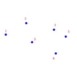
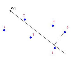
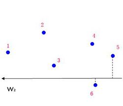
The points generated by the training data are in the feature space, which also carry the rank information (the labels). These labeled points can be used to find the boundary (classifier) that specifies the order of them. In the linear case, such boundary (classifier) is a vector.

Suppose [math]\displaystyle{ c_i }[/math] and [math]\displaystyle{ c_j }[/math] are two elements in the database and denote [math]\displaystyle{ (c_i,c_j) \in r }[/math] if the rank of [math]\displaystyle{ c_i }[/math] is higher than [math]\displaystyle{ c_j }[/math] in certain ranking method [math]\displaystyle{ r }[/math]. Let vector [math]\displaystyle{ \vec w }[/math] be the linear classifier candidate in the feature space. Then the ranking problem can be translated to the following SVM classification problem. Note that one ranking method corresponds to one query.

[math]\displaystyle{ \begin{align} & \text{minimize } V(\vec w, \vec \xi) = {1 \over 2} \vec w \cdot \vec w + \text{constant} \cdot \sum \xi_{i,j,k} \\[6pt] & \text{subject to} \\[6pt] & \begin{array}{l} \forall \xi_{i,j,k} \geqq 0\\ \forall (c_i, c_j)\in r_k^*\\ \vec w (\Phi(q_1,c_i)-\Phi(q_1, c_j)) \geqq 1- \xi_{i,j,1};\\ \,\,\,\vdots \\ \vec w (\Phi(q_n, c_i)-\Phi(q_n, c_j)) \geqq 1-\xi_{i,j,n};\\ \text{where } k \in \left \{ 1,2,\ldots, n \right \},\ i,j \in \left \{ 1,2,\ldots \right \}. \end{array} \end{align} }[/math]

The above optimization problem is identical to the classical SVM classification problem, which is the reason why this algorithm is called Ranking-SVM.

W candidate

Not a w candidate

Retrieval function

The optimal vector [math]\displaystyle{ \vec w^* }[/math] obtained by the training sample is

[math]\displaystyle{ \vec w^*=\sum \alpha_{k,\ell}^*\Phi(q_k,c_i) }[/math]

So the retrieval function could be formed based on such optimal classifier.
For new query [math]\displaystyle{ q }[/math], the retrieval function first projects all elements of the database to the feature space. Then it orders these feature points by the values of their inner products with the optimal vector. And the rank of each feature point is the rank of the corresponding element of database for the query [math]\displaystyle{ q }[/math].

Application of ranking SVM

Ranking SVM can be applied to rank the pages according to the query. The algorithm can be trained using click-through data, where consists of the following three parts:

1. Query.
2. Present ranking of search results
3. Search results clicked on by user

The combination of 2 and 3 cannot provide full training data order which is needed to apply the full SVM algorithm. Instead, it provides a part of the ranking information of the training data. So the algorithm can be slightly revised as follows.

[math]\displaystyle{ \begin{align} & \text{minimize } V(\vec w, \vec \xi) = {1 \over 2} \vec w \cdot \vec w + \text{constant} \cdot \sum \xi_{i,j,k} \\[6pt] & \text{subject to} \\[6pt] & \begin{array}{l} \forall \xi_{i,j,k} \geqq 0\\ \forall (c_i, c_j)\in r_k'\\ \vec w (\Phi(q_1,c_i)-\Phi(q_1,c_j)) \geqq 1- \xi_{i,j,1};\\ \,\,\, \vdots \\ \vec w (\Phi(q_n,c_i)-\Phi(q_n,c_j)) \geqq 1- \xi_{i,j,n};\\ \text{where }\ k \in \left \{ 1,2,\ldots,n \right \},\ i,j \in \left \{ 1,2,\ldots \right \}. \end{array} \end{align} }[/math]

The method [math]\displaystyle{ r' }[/math] does not provide ranking information of the whole dataset, it's a subset of the full ranking method. So the condition of optimization problem becomes more relax compared with the original Ranking-SVM.

References

- ↑ Joachims, T. (2002), "Optimizing Search Engines using Clickthrough Data", Proceedings of the ACM Conference on Knowledge Discovery and Data Mining
- ↑ Bing Li; Rong Xiao; Zhiwei Li; Rui Cai; Bao-Liang Lu; Lei Zhang; "Rank-SIFT: Learning to rank repeatable local interest points", Computer Vision and Pattern Recognition (CVPR), 2011
- ↑ M. Kemeny. Rank Correlation Methods, Hafner, 1955
- ↑ A. Mood, F. Graybill, and D. Boes. Introduction to the Theory of Statistics. McGraw-Hill, 3rd edition, 1974
- ↑ J. Kemeny and L. Snell. Mathematical Models in THE Social Sciences. Ginn & Co. 1962
- ↑ Y. Yao. "Measuring retrieval effectiveness based on user preference of documents." Journal of the American Society for Information Science, 46(2): 133–145, 1995.
- ↑ R. Baeza-Yates and B. Ribeiro-Neto. Modern Information Retrieval. Addison-Wesley-Longman, Harlow, UK, May 1999
- ↑ C. Cortes and V.N. Vapnik. "Support-vector networks." Machine Learning Journal, 20: 273–297,1995
- ↑ V. Vapnik. Statistical Learning Theory. WILEY, Chichester, GB, 1998
- ↑ N. Fuhr. "Optimum polynomial retrieval functions based on the probability ranking principle." ACM TRANSACTIONS on Information Systems, 7(3): 183–204
- ↑ N. Fuhr, S. Hartmann, G. Lustig, M. Schwantner, K. Tzeras, and G. Knorz. "Air/x – a rule-based multistage indexing system for large subject fields." In RIAO, 1991