Biology:Felsenstein's tree-pruning algorithm

Short description: Technique in statistical genetics

In statistical genetics, Felsenstein's tree-pruning algorithm (or Felsenstein's tree-peeling algorithm), attributed to Joseph Felsenstein, is an algorithm for efficiently computing the likelihood of an evolutionary tree from nucleic acid sequence data.

The algorithm is often used as a subroutine in a search for a maximum likelihood estimate for an evolutionary tree. Further, it can be used in a hypothesis test for whether evolutionary rates are constant (by using likelihood ratio tests). It can also be used to provide error estimates for the parameters describing an evolutionary tree.

Details

A simple phylogenetic tree exemple made from arbitrary data D

The likelihood of a tree [math]\displaystyle{ T }[/math] is, by definition, the probability of observing certain data [math]\displaystyle{ D }[/math] ([math]\displaystyle{ D }[/math] being a nucleotide sequence alignment for example i.e. a succession of [math]\displaystyle{ n }[/math] DNA site [math]\displaystyle{ s }[/math]) given the tree. It is often written : [math]\displaystyle{ P(D|T) }[/math].

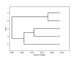
Here is an example of an evolutionary tree on arbitrary sequence data [math]\displaystyle{ D }[/math]:

This is a key value and is often quite complicated to compute. To ease the computations, Felsenstein and his colleagues used several assumptions that are still widely used today. The main assumption is that mutations between DNA sites are independant of each other. This permits to compute the likelihood as a simple product of probabilities. Now you can divide the data [math]\displaystyle{ D }[/math] between several [math]\displaystyle{ D_s }[/math] for each nucleotide site [math]\displaystyle{ s }[/math] inside of [math]\displaystyle{ D }[/math]. The global likelihood of the tree will be the product of the likelihoods of each site:

Same tree but made from D1, which consists in the first DNA sites from D

[math]\displaystyle{ P(D|T) = \prod_{s=1}^{n} {P(D_s|T)} }[/math]

If I reuse the exemple above, [math]\displaystyle{ D_1 }[/math] tree would be:

The second assumption concerns the models of DNA sequence evolution. The computation of the likelihood needs the nucleotide frequencies as well as the transition probabilities (when a mutation occurs, probability of going from a nucleotide to another). The simplest model is the Jukes-Cantor model, assuming equal nucleotide frequencies [math]\displaystyle{ \left(\pi_A = \pi_G = \pi_C = \pi_T = {1\over4}\right) }[/math] and equal transition probabilities from [math]\displaystyle{ X }[/math] to [math]\displaystyle{ Y }[/math] ([math]\displaystyle{ p_{A \rightarrow T} = p_{A \rightarrow C} = p_{A \rightarrow G} = \frac{1}{4} (1 - e^{-\mu l}) }[/math] and [math]\displaystyle{ p_{A \rightarrow A} = e^{-\mu l} + \frac{1}{4} (1 - e^{-\mu l}) }[/math]) and idem for the other bases. Here [math]\displaystyle{ \mu }[/math] is the global mutation rate of the model.

Felsenstein proposed to decomposed computations even more by using "partial likelihoods" in the computation of [math]\displaystyle{ P( D_s | T) }[/math]. Here is how it works.

Assume we are on a node [math]\displaystyle{ k }[/math] on the tree [math]\displaystyle{ T }[/math]. [math]\displaystyle{ k }[/math] has two daughter nodes [math]\displaystyle{ i }[/math] and [math]\displaystyle{ j }[/math] and, for each DNA base [math]\displaystyle{ X = \{ A, T, C, G \} }[/math] present on [math]\displaystyle{ k }[/math], we can define a partial likelihood [math]\displaystyle{ w_k (X) }[/math] such as:

[math]\displaystyle{ w_k (X) = ( \sum_Y p_{X \rightarrow Y} \centerdot w_i (Y)) \centerdot ( \sum_Z p_{X \rightarrow Z} \centerdot w_j (Z)) }[/math]

where [math]\displaystyle{ Y }[/math] and [math]\displaystyle{ Z }[/math] are also DNA bases. [math]\displaystyle{ p_{ X\rightarrow Y} }[/math]is the transition probability from nucleotide [math]\displaystyle{ X }[/math] to nucleotide [math]\displaystyle{ Y }[/math] (idem for [math]\displaystyle{ p_{X \rightarrow Z} }[/math]). [math]\displaystyle{ w_i(Y) }[/math] is the partial likelihood of the daughter node [math]\displaystyle{ i }[/math], evaluated on nucleotide [math]\displaystyle{ Y }[/math] (idem for [math]\displaystyle{ w_j(Z) }[/math]).

Using this formula, one has to start from the tips of the tree [math]\displaystyle{ T }[/math], then move towards the root and compute the partial likelihoods of each necessary node on the way (4 partial likelihoods per node). Having finished at the root of the tree, the likelihood of the tree (for this particular site) is then the sum of the partial likelihoods of the root times the appropriated nucleotide frequency.

[math]\displaystyle{ P(D_s|T) = \sum_X p_X \centerdot w_r (X) }[/math]

After doing so for every site [math]\displaystyle{ s }[/math], one can finally obtain the likelihood of the global evolutionary tree by multiplying each "sublikelihood".

References

- ↑ Felsenstein, J. (1973). "Maximum Likelihood and Minimum-Steps Methods for Estimating Evolutionary Trees from Data on Discrete Characters". Systematic Biology 22 (3): 240–249. doi:10.1093/sysbio/22.3.240.
- ↑ Felsenstein, J. (1981). "Evolutionary trees from DNA sequences: A maximum likelihood approach". Journal of Molecular Evolution 17 (6): 368–376. doi:10.1007/BF01734359. PMID 7288891. Bibcode: 1981JMolE..17..368F.