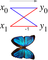
Butterfly diagram

In the context of fast Fourier transform algorithms, a butterfly is a portion of the computation that combines the results of smaller discrete Fourier transforms (DFTs) into a larger DFT, or vice versa (breaking a larger DFT up into subtransforms). The name "butterfly" comes from the shape of the data-flow diagram in the radix-2 case, as described below.[1] The earliest occurrence in print of the term is thought to be in a 1969 MIT technical report.[2][3] The same structure can also be found in the Viterbi algorithm, used for finding the most likely sequence of hidden states.
Most commonly, the term "butterfly" appears in the context of the Cooley–Tukey FFT algorithm, which recursively breaks down a DFT of composite size n = rm into r smaller transforms of size m where r is the "radix" of the transform. These smaller DFTs are then combined via size-r butterflies, which themselves are DFTs of size r (performed m times on corresponding outputs of the sub-transforms) pre-multiplied by roots of unity (known as twiddle factors). (This is the "decimation in time" case; one can also perform the steps in reverse, known as "decimation in frequency", where the butterflies come first and are post-multiplied by twiddle factors. See also the Cooley–Tukey FFT article.)
Radix-2 butterfly diagram
In the case of the radix-2 Cooley–Tukey algorithm, the butterfly is simply a DFT of size-2 that takes two inputs (x0, x1) (corresponding outputs of the two sub-transforms) and gives two outputs (y0, y1) by the formula (not including twiddle factors):
If one draws the data-flow diagram for this pair of operations, the (x0, x1) to (y0, y1) lines cross and resemble the wings of a butterfly, hence the name (see also the illustration at right).

More specifically, a radix-2 decimation-in-time FFT algorithm on n = 2 p inputs with respect to a primitive n-th root of unity relies on O(n log2 n) butterflies of the form:
where k is an integer depending on the part of the transform being computed. Whereas the corresponding inverse transform can mathematically be performed by replacing ω with ω−1 (and possibly multiplying by an overall scale factor, depending on the normalization convention), one may also directly invert the butterflies:
corresponding to a decimation-in-frequency FFT algorithm.
Other uses
The butterfly can also be used to improve the randomness of large arrays of partially random numbers, by bringing every 32 or 64 bit word into causal contact with every other word through a desired hashing algorithm, so that a change in any one bit has the possibility of changing all the bits in the large array.[4]
See also
References
- ↑ Alan V. Oppenheim, Ronald W. Schafer, and John R. Buck, Discrete-Time Signal Processing, 2nd edition (Upper Saddle River, NJ: Prentice Hall, 1989)
- ↑ C. J. Weinstein (1969-11-21). Quantization Effects in Digital Filters (Report). MIT Lincoln Laboratory. p. 42. https://www.ll.mit.edu/sites/default/files/publication/doc/quantization-effects-digital-filters-weinstein-tr-468.pdf. "This computation, referred to as a 'butterfly'"
- ↑ Cipra, Barry A. (2012-06-04). "FFT and Butterfly Diagram". https://mathoverflow.net/q/98804.
- ↑ Press, William H.; Teukolsky, Saul A.; Vetterling, William T.; Flannery, Brian P. (2007), "Section 7.2 Completely Hashing a Large Array", Numerical Recipes: The Art of Scientific Computing (3rd ed.), New York: Cambridge University Press, pp. 358, ISBN 978-0-521-88068-8, https://www.cambridge.org/ru/universitypress/subjects/mathematics/numerical-recipes/numerical-recipes-art-scientific-computing-3rd-edition
External links
- explanation of the FFT and butterfly diagrams.
- butterfly diagrams of various FFT implementations (Radix-2, Radix-4, Split-Radix).
 |
