Composite Bézier curve

Short description: Geometric shape

Beziergon – The red beziergon passes through the blue vertices, the green points are control points that determine the shape of the connecting Bézier curves

In geometric modelling and in computer graphics, a composite Bézier curve or Bézier spline is a spline made out of Bézier curves that is at least [math]\displaystyle{ C^0 }[/math] continuous. In other words, a composite Bézier curve is a series of Bézier curves joined end to end where the last point of one curve coincides with the starting point of the next curve. Depending on the application, additional smoothness requirements (such as [math]\displaystyle{ C^1 }[/math] or [math]\displaystyle{ C^2 }[/math] continuity) may be added.

A continuous composite Bézier is also called a polybezier, by similarity to polyline, but whereas in polylines the points are connected by straight lines, in a polybezier the points are connected by Bézier curves. A beziergon (also called bezigon) is a closed path composed of Bézier curves. It is similar to a polygon in that it connects a set of vertices by lines, but whereas in polygons the vertices are connected by straight lines, in a beziergon the vertices are connected by Bézier curves. Some authors even call a [math]\displaystyle{ C^0 }[/math] composite Bézier curve a "Bézier spline"; the latter term is however used by other authors as a synonym for the (non-composite) Bézier curve, and they add "composite" in front of "Bézier spline" to denote the composite case.

Perhaps the most common use of composite Béziers is to describe the outline of each letter in a PostScript or PDF file. Such outlines are composed of one beziergon for open letters, or multiple beziergons for closed letters. Modern vector graphics and computer font systems like PostScript, Asymptote, Metafont, OpenType, and SVG use composite Bézier curves composed of cubic Bézier curves (3rd order curves) for drawing curved shapes.

Sinc function approximated using a smooth Bézier spline, i.e., a series of smoothly-joined Bézier curves

Smooth joining

A commonly desired property of splines is for them to join their individual curves together with a specified level of parametric or geometric continuity. While individual curves in the spline are fully [math]\displaystyle{ C^\infin }[/math] continuous within their own interval, there is always some amount of discontinuity where different curves meet.

The Bézier spline is fairly unique in that it's one of the few splines that doesn't guarantee any higher degree of continuity than [math]\displaystyle{ C^0 }[/math]. It is, however, possible to arrange control points to guarantee various levels of continuity across joins, though this can come at a loss of local control if the constraint is too strict for the given degree of the Bézier spline.

Smoothly joining cubic Béziers

Given two cubic Bézier curves with control points [math]\displaystyle{ [\mathbf P_0,\mathbf P_1,\mathbf P_2,\mathbf P_3] }[/math] and [math]\displaystyle{ [\mathbf P_3,\mathbf P_4,\mathbf P_5,\mathbf P_6] }[/math] respectively, the constraints for ensuring continuity at [math]\displaystyle{ \mathbf P_3 }[/math] can be defined as follows:

• [math]\displaystyle{ C^0/G^0 }[/math] (positional continuity) requires that they meet at the same point, which all Bézier splines do by definition. In this example, the shared point is [math]\displaystyle{ \mathbf P_3 }[/math]

• [math]\displaystyle{ C^1 }[/math] (velocity continuity) requires the neighboring control points around the join to be mirrors of each other. In other words, they must follow the constraint of [math]\displaystyle{ \mathbf P_4=2\mathbf P_3-\mathbf P_2 }[/math]

• [math]\displaystyle{ G^1 }[/math] (tangent continuity) requires the neighboring control points to be collinear with the join. This is less strict than [math]\displaystyle{ C^1 }[/math] continuity, leaving an extra degree of freedom which can be parameterized using a scalar [math]\displaystyle{ \beta_1 }[/math]. The constraint can then be expressed by [math]\displaystyle{ \mathbf P_4=\mathbf P_3+(\mathbf P_3-\mathbf P_2)\beta_1 }[/math]

While the following continuity constraints are possible, they are rarely used with cubic Bézier splines, as other splines like the B-spline or the β-spline will naturally handle higher constraints without loss of local control.

• [math]\displaystyle{ C^2 }[/math] (acceleration continuity) is constrained by [math]\displaystyle{ \mathbf P_5 =\mathbf P_1+4(\mathbf P_3-\mathbf P_2) }[/math]. However, applying this constraint across an entire cubic Bézier spline will cause a cascading loss of local control over the tangent points. The curve will still pass through every third point in the spline, but control over its shape will be lost. In order to achieve [math]\displaystyle{ C^2 }[/math] continuity using cubic curves, it's recommended to use a cubic uniform B-spline instead, as it ensures [math]\displaystyle{ C^2 }[/math] continuity without loss of local control, at the expense of no longer being guaranteed to pass through specific points

• [math]\displaystyle{ G^2 }[/math] (curvature continuity) is constrained by [math]\displaystyle{ \mathbf P_5=\mathbf P_3+(\mathbf P_3-\mathbf P_2)(2\beta_1+\beta_1^2+\beta_2/2)+(\mathbf P_1-\mathbf P_2)\beta_1^2 }[/math], leaving two degrees of freedom compared to [math]\displaystyle{ C^2 }[/math], in the form of two scalars [math]\displaystyle{ \beta_1 }[/math] and [math]\displaystyle{ \beta_2 }[/math]. Higher degrees of geometric continuity is possible, though they get increasingly complex

• [math]\displaystyle{ C^3 }[/math] (jolt continuity) is constrained by [math]\displaystyle{ \mathbf P_6=\mathbf P_3+(\mathbf P_3-\mathbf P_0)+6(\mathbf P_1-\mathbf P_2+\mathbf P_3-\mathbf P_2) }[/math]. Applying this constraint to the cubic Bézier spline will cause a complete loss of local control, as the entire spline is now fully constrained and defined by the first curve's control points. In fact, it is arguably no longer a spline, as its shape is now equivalent to extrapolating the first curve indefinitely, making it not only [math]\displaystyle{ C^3 }[/math] continuous, but [math]\displaystyle{ C^\infin }[/math], as joins between separate curves no longer exist

Approximating circular arcs

In case circular arc primitives are not supported in a particular environment, they may be approximated by Bézier curves. Commonly, eight quadratic segments or four cubic segments are used to approximate a circle. It is desirable to find the length [math]\displaystyle{ \mathbf{k} }[/math] of control points which result in the least approximation error for a given number of cubic segments.

Using four curves

Considering only the 90-degree unit-circular arc in the first quadrant, we define the endpoints [math]\displaystyle{ \mathbf{A} }[/math] and [math]\displaystyle{ \mathbf{B} }[/math] with control points [math]\displaystyle{ \mathbf{A'} }[/math] and [math]\displaystyle{ \mathbf{B'} }[/math], respectively, as:

[math]\displaystyle{ \begin{align} \mathbf{A} & = [0, 1] \\ \mathbf{A'} & = [\mathbf{k}, 1] \\ \mathbf{B'} & = [1, \mathbf{k}] \\ \mathbf{B} & = [1, 0] \\ \end{align} }[/math]

From the definition of the cubic Bézier curve, we have:

[math]\displaystyle{ \mathbf{C}(t)=(1-t)^3\mathbf{A} + 3(1-t)^2t\mathbf{A'}+3(1-t)t^2\mathbf{B'}+t^3\mathbf{B} }[/math]

With the point [math]\displaystyle{ \mathbf{C}(t=0.5) }[/math] as the midpoint of the arc, we may write the following two equations:

[math]\displaystyle{ \begin{align} \mathbf{C} &= \frac{1}{8}\mathbf{A} + \frac{3}{8}\mathbf{A'}+\frac{3}{8}\mathbf{B'}+\frac{1}{8}\mathbf{B} \\ \mathbf{C} &= \sqrt{1/2} = \sqrt{2}/2 \end{align} }[/math]

Solving these equations for the x-coordinate (and identically for the y-coordinate) yields:

[math]\displaystyle{ \frac{0}{8}\mathbf + \frac{3}{8}\mathbf{k}+\frac{3}{8} + \frac{1}{8} = \sqrt{2}/2 }[/math]

[math]\displaystyle{ \mathbf{k} = \frac{4}{3}(\sqrt{2} - 1) \approx 0.5522847498 }[/math]

Note however that the resulting Bézier curve is entirely outside the circle, with a maximum deviation of the radius of about 0.00027. By adding a small correction to intermediate points such as

[math]\displaystyle{ \begin{align} \mathbf{A'} & = [\mathbf{k}+0.0009, 1-0.00103] \\ \mathbf{B'} & = [1-0.00103, \mathbf{k}+0.0009] , \end{align} }[/math]

the magnitude of the radius deviation to 1 is reduced by a factor of about 3, to 0.000068 (at the expense of the derivability of the approximated circle curve at endpoints).

General case

We may compose a circle of radius [math]\displaystyle{ R }[/math] from an arbitrary number of cubic Bézier curves. Let the arc start at point [math]\displaystyle{ \mathbf{A} }[/math] and end at point [math]\displaystyle{ \mathbf{B} }[/math], placed at equal distances above and below the x-axis, spanning an arc of angle [math]\displaystyle{ \theta = 2\phi }[/math]:

[math]\displaystyle{ \begin{align} \mathbf{A}_x &= R\cos(\phi) \\ \mathbf{A}_y &= R\sin(\phi) \\ \mathbf{B}_x &= \mathbf{A}_x \\ \mathbf{B}_y &= -\mathbf{A}_y \end{align} }[/math]

The control points may be written as:

[math]\displaystyle{ \begin{align} \mathbf{A'}_x &= \frac{4R - \mathbf{A}_x}{3} \\ \mathbf{A'}_y &= \frac{(R - \mathbf{A}_x)(3R - \mathbf{A}_x)}{3\mathbf{A}_y} \\ \mathbf{B'}_x &= \mathbf{A'}_x \\ \mathbf{B'}_y &= -\mathbf{A'}_y \end{align} }[/math]

Examples

• 

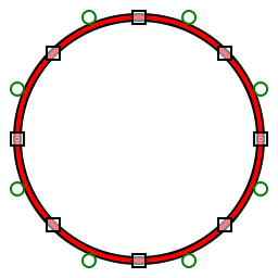
  Eight-segment quadratic polybezier (red) approximating a circle (black) with control points

• 

  Four-segment cubic polybezier (red) approximating a circle (black) with control points

Fonts

TrueType fonts use composite Béziers composed of quadratic Bézier curves (2nd order curves). To describe a typical type design as a computer font to any given accuracy, 3rd order Beziers require less data than 2nd order Beziers; and these in turn require less data than a series of straight lines. This is true even though any one straight line segment requires less data than any one segment of a parabola; and that parabolic segment in turn requires less data than any one segment of a 3rd order curve.

See also

• B-spline

References

- ↑ Eugene V. Shikin; Alexander I. Plis (14 July 1995). Handbook on Splines for the User. CRC Press. p. 96. ISBN 978-0-8493-9404-1. https://books.google.com/books?id=DL88KouJCQkC&pg=PA96.
- ↑ Microsoft polybezier API
- ↑ Papyrus beziergon API reference
- ↑ "A better box of crayons". InfoWorld. 1991.
- ↑ Rebaza, Jorge (2012-04-24) (in en). A First Course in Applied Mathematics. John Wiley & Sons. ISBN 9781118277157. https://books.google.com/books?id=lFwXglfyoIQC.
- ↑ (Firm), Wolfram Research (1996-09-13) (in en). Mathematica ® 3.0 Standard Add-on Packages. Cambridge University Press. ISBN 9780521585859. https://books.google.com/books?id=VnH0UzTycTcC.
- ↑ Goodman, T.N.T (1983-12-09). "Properties of β-splines" (in en). Journal of Approximation Theory 44 (2): 132–153. doi:10.1016/0021-9045(85)90076-0.
- ↑ DeRose, Anthony D. (1985-08-01). "Geometric Continuity: A Parametrization Independent Measure of Continuity for Computer Aided Geometric Design" (in en). https://www2.eecs.berkeley.edu/Pubs/TechRpts/1986/6081.html.
- ↑ Stanislav, G. Adam. "Drawing a circle with Bézier Curves". http://whizkidtech.redprince.net/bezier/circle/. Retrieved 10 April 2010.
- ↑ "Digitizing letterform designs". Apple. https://developer.apple.com/fonts/ttrefman/RM01/Chap1.html. Retrieved 26 July 2014.
- ↑ Riškus, Aleksas (October 2006). "APPROXIMATION OF A CUBIC BEZIER CURVE BY CIRCULAR ARCS AND VICE VERSA". Information Technology and Control (Department of Multimedia Engineering, Kaunas University of Technology) 35 (4): 371–378. ISSN 1392-124X. https://people-mozilla.org/~jmuizelaar/Riskus354.pdf.
- ↑ DeVeneza, Richard. "Drawing a circle with Bézier Curves". http://www.tinaja.com/glib/bezcirc2.pdf. Retrieved 10 April 2010.