Continuous analogues of iteration methods

Continuous models that make it possible to study problems concerning the existence of solutions of non-linear equations, to produce by means of the well-developed apparatus of continuous analysis preliminary results on the convergence and optimality of iteration methods, and to obtain new classes of such methods.

One can set up a correspondence between methods for solving stationary problems by adjustment (see Adjustment method) and certain iteration methods (see [1], [2]). For example, for the solution of a linear equation

<img align="absmiddle" border="0" src="https://www.encyclopediaofmath.org/legacyimages/c/c025/c025600/c0256001.png" />

(1)

with a positive-definite self-adjoint operator <img align="absmiddle" border="0" src="https://www.encyclopediaofmath.org/legacyimages/c/c025/c025600/c0256002.png" /> it is known that one-step iteration methods of the form

<img align="absmiddle" border="0" src="https://www.encyclopediaofmath.org/legacyimages/c/c025/c025600/c0256003.png" />

(2)

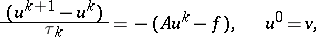
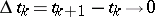
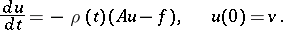
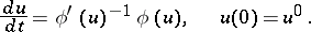
converge for sufficiently small <img align="absmiddle" border="0" src="https://www.encyclopediaofmath.org/legacyimages/c/c025/c025600/c0256004.png" />. Introduce a continuous time <img align="absmiddle" border="0" src="https://www.encyclopediaofmath.org/legacyimages/c/c025/c025600/c0256005.png" /> and regard the quantities <img align="absmiddle" border="0" src="https://www.encyclopediaofmath.org/legacyimages/c/c025/c025600/c0256006.png" /> as the values of a certain function <img align="absmiddle" border="0" src="https://www.encyclopediaofmath.org/legacyimages/c/c025/c025600/c0256007.png" /> at <img align="absmiddle" border="0" src="https://www.encyclopediaofmath.org/legacyimages/c/c025/c025600/c0256008.png" />, where

<img align="absmiddle" border="0" src="https://www.encyclopediaofmath.org/legacyimages/c/c025/c025600/c0256009.png" />

If one puts <img align="absmiddle" border="0" src="https://www.encyclopediaofmath.org/legacyimages/c/c025/c025600/c02560010.png" />, where <img align="absmiddle" border="0" src="https://www.encyclopediaofmath.org/legacyimages/c/c025/c025600/c02560011.png" /> is a continuous function for <img align="absmiddle" border="0" src="https://www.encyclopediaofmath.org/legacyimages/c/c025/c025600/c02560012.png" />, then in passing to the limit in (2) as <img align="absmiddle" border="0" src="https://www.encyclopediaofmath.org/legacyimages/c/c025/c025600/c02560013.png" />, one obtains a continuous analogue of the iteration method (2):

<img align="absmiddle" border="0" src="https://www.encyclopediaofmath.org/legacyimages/c/c025/c025600/c02560014.png" />

(3)

If also

<img align="absmiddle" border="0" src="https://www.encyclopediaofmath.org/legacyimages/c/c025/c025600/c02560015.png" />

as <img align="absmiddle" border="0" src="https://www.encyclopediaofmath.org/legacyimages/c/c025/c025600/c02560016.png" />, then <img align="absmiddle" border="0" src="https://www.encyclopediaofmath.org/legacyimages/c/c025/c025600/c02560017.png" /> tends to <img align="absmiddle" border="0" src="https://www.encyclopediaofmath.org/legacyimages/c/c025/c025600/c02560018.png" />, a solution of (1).

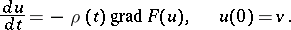
Similarly, with the one-step gradient iteration methods for the minimization of a function <img align="absmiddle" border="0" src="https://www.encyclopediaofmath.org/legacyimages/c/c025/c025600/c02560019.png" />:

<img align="absmiddle" border="0" src="https://www.encyclopediaofmath.org/legacyimages/c/c025/c025600/c02560020.png" />

(4)

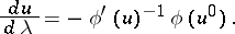
one can associate a continuous analogue:

<img align="absmiddle" border="0" src="https://www.encyclopediaofmath.org/legacyimages/c/c025/c025600/c02560021.png" />

(5)

Here the function <img align="absmiddle" border="0" src="https://www.encyclopediaofmath.org/legacyimages/c/c025/c025600/c02560022.png" /> affects only the parametrization of the curve of steepest descent. To solve (1) one may take <img align="absmiddle" border="0" src="https://www.encyclopediaofmath.org/legacyimages/c/c025/c025600/c02560023.png" />. Then the formulas (4) take the form (2) and the equations (5) the form (3).

By means of transformations two-step iteration methods

<img align="absmiddle" border="0" src="https://www.encyclopediaofmath.org/legacyimages/c/c025/c025600/c02560024.png" />

(6)

can be brought to the form

<img align="absmiddle" border="0" src="https://www.encyclopediaofmath.org/legacyimages/c/c025/c025600/c02560025.png" />

(7)

<img align="absmiddle" border="0" src="https://www.encyclopediaofmath.org/legacyimages/c/c025/c025600/c02560026.png" />

where the quantities <img align="absmiddle" border="0" src="https://www.encyclopediaofmath.org/legacyimages/c/c025/c025600/c02560027.png" />, and <img align="absmiddle" border="0" src="https://www.encyclopediaofmath.org/legacyimages/c/c025/c025600/c02560028.png" /> are (non-uniquely) defined in terms of the parameters <img align="absmiddle" border="0" src="https://www.encyclopediaofmath.org/legacyimages/c/c025/c025600/c02560029.png" /> and <img align="absmiddle" border="0" src="https://www.encyclopediaofmath.org/legacyimages/c/c025/c025600/c02560030.png" /> of (6). Taking limits in (7) as <img align="absmiddle" border="0" src="https://www.encyclopediaofmath.org/legacyimages/c/c025/c025600/c02560031.png" /> leads to a continuous analogue:

<img align="absmiddle" border="0" src="https://www.encyclopediaofmath.org/legacyimages/c/c025/c025600/c02560032.png" />

(8)

The adjustment method involving an equation like (8) is called the method of the heavy sphere (see [2]). There exist iteration methods for which the continuous analogues contain differential operators of higher orders (see [3]).

A source for obtaining differential equations playing the role of continuous analogues of iteration methods can be the continuation method (with respect to a parameter) (see [4], [5]). In this method, to find a solution of an equation

<img align="absmiddle" border="0" src="https://www.encyclopediaofmath.org/legacyimages/c/c025/c025600/c02560033.png" />

(9)

one constructs an equation

<img align="absmiddle" border="0" src="https://www.encyclopediaofmath.org/legacyimages/c/c025/c025600/c02560034.png" />

(10)

depending on a parameter <img align="absmiddle" border="0" src="https://www.encyclopediaofmath.org/legacyimages/c/c025/c025600/c02560035.png" />, such that for <img align="absmiddle" border="0" src="https://www.encyclopediaofmath.org/legacyimages/c/c025/c025600/c02560036.png" /> a solution of (10) is known: <img align="absmiddle" border="0" src="https://www.encyclopediaofmath.org/legacyimages/c/c025/c025600/c02560037.png" />, and such that for <img align="absmiddle" border="0" src="https://www.encyclopediaofmath.org/legacyimages/c/c025/c025600/c02560038.png" /> the solutions of (9) and (10) are the same. For example, one can take

<img align="absmiddle" border="0" src="https://www.encyclopediaofmath.org/legacyimages/c/c025/c025600/c02560039.png" />

(11)

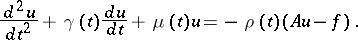
By differentiating (1) with respect to the parameter and taking <img align="absmiddle" border="0" src="https://www.encyclopediaofmath.org/legacyimages/c/c025/c025600/c02560040.png" /> one obtains a differential equation for <img align="absmiddle" border="0" src="https://www.encyclopediaofmath.org/legacyimages/c/c025/c025600/c02560041.png" />; for the case (11) it takes the form

<img align="absmiddle" border="0" src="https://www.encyclopediaofmath.org/legacyimages/c/c025/c025600/c02560042.png" />

(12)

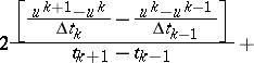
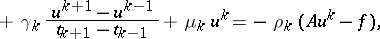
By splitting the interval <img align="absmiddle" border="0" src="https://www.encyclopediaofmath.org/legacyimages/c/c025/c025600/c02560043.png" /> into <img align="absmiddle" border="0" src="https://www.encyclopediaofmath.org/legacyimages/c/c025/c025600/c02560044.png" /> parts by points <img align="absmiddle" border="0" src="https://www.encyclopediaofmath.org/legacyimages/c/c025/c025600/c02560045.png" /> and using for (12) a numerical discretization formula at the points <img align="absmiddle" border="0" src="https://www.encyclopediaofmath.org/legacyimages/c/c025/c025600/c02560046.png" /> (e.g., Euler's method, the Runge–Kutta method, etc.), one obtains recurrence relations between the quantities <img align="absmiddle" border="0" src="https://www.encyclopediaofmath.org/legacyimages/c/c025/c025600/c02560047.png" />, which one uses to construct the formulas of an iteration method. Thus, after e.g. applying Euler's method, (12) is replaced by the relations

<img align="absmiddle" border="0" src="https://www.encyclopediaofmath.org/legacyimages/c/c025/c025600/c02560048.png" />

(13)

where <img align="absmiddle" border="0" src="https://www.encyclopediaofmath.org/legacyimages/c/c025/c025600/c02560049.png" />, which determine the following two-step iteration method containing internal and external iteration cycles:

<img align="absmiddle" border="0" src="https://www.encyclopediaofmath.org/legacyimages/c/c025/c025600/c02560050.png" />

(14)

<img align="absmiddle" border="0" src="https://www.encyclopediaofmath.org/legacyimages/c/c025/c025600/c02560051.png" />

For <img align="absmiddle" border="0" src="https://www.encyclopediaofmath.org/legacyimages/c/c025/c025600/c02560052.png" /> and <img align="absmiddle" border="0" src="https://www.encyclopediaofmath.org/legacyimages/c/c025/c025600/c02560053.png" /> this turns into Newton's classical method. A continuous analogue of Newton's iteration method can also be obtained in another way: In (11) the variable is replaced by <img align="absmiddle" border="0" src="https://www.encyclopediaofmath.org/legacyimages/c/c025/c025600/c02560054.png" />. Then the differential equation (12) takes the form

<img align="absmiddle" border="0" src="https://www.encyclopediaofmath.org/legacyimages/c/c025/c025600/c02560055.png" />

(15)

Numerical integration of (15) by Euler's method with respect to the points <img align="absmiddle" border="0" src="https://www.encyclopediaofmath.org/legacyimages/c/c025/c025600/c02560056.png" /> leads to the iteration method

<img align="absmiddle" border="0" src="https://www.encyclopediaofmath.org/legacyimages/c/c025/c025600/c02560057.png" />

which coincides for <img align="absmiddle" border="0" src="https://www.encyclopediaofmath.org/legacyimages/c/c025/c025600/c02560058.png" /> with Newton's classical method.

Continuous analogues of iteration methods for the solution of boundary value problems for the differential equations of mathematical physics are, as a rule, mixed problems for partial differential equations of a special form (e.g. with rapidly oscillating coefficients or with small coefficients in front of the highest derivatives).

See also Closure of a computational algorithm.

References

[1]	M.K. Gavurin, "Nonlinear functional equations and continuous analogues of iteration methods" Izv. Vyssh. Uchevn. Zaved. Mat. : 5 (6) (1958) pp. 18–31 (In Russian)
[2]	N.S. Bakhvalov, "Numerical methods: analysis, algebra, ordinary differential equations" , 1 , MIR (1977) (Translated from Russian)
[3]	G.I. Marchuk, V.I. Lebedev, "Numerical methods in the theory of neutron transport" , Harwood (1986) (Translated from Russian)
[4]	J.M. Ortega, W.C. Rheinboldt, "Iterative solution of nonlinear equations in several variables" , Acad. Press (1970)
[5]	D.F. Davidenko, "The iteration method of parameter variation for the inversion of linear operations" Zh. Vychisl. Mat. i. Mat. Fiz. , 15 : 1 (1975) pp. 30–47 (In Russian)

References

[a1]	W.C. Rheinboldt, "Numerical analysis of parametrized nonlinear equations" , Wiley (1986)