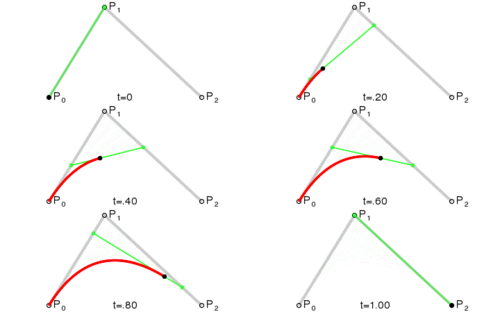
De Casteljau's algorithm
In the mathematical field of numerical analysis, De Casteljau's algorithm is a recursive method to evaluate polynomials in Bernstein form or Bézier curves, named after its inventor Paul de Casteljau. De Casteljau's algorithm can also be used to split a single Bézier curve into two Bézier curves at an arbitrary parameter value. Although the algorithm is slower for most architectures when compared with the direct approach, it is more numerically stable.[citation needed]
Definition
A Bézier curve (of degree , with control points ) can be written in Bernstein form as follows
where is a Bernstein basis polynomial
The curve at point can be evaluated with the recurrence relation
Then, the evaluation of at point can be evaluated in operations. The result is given by
Moreover, the Bézier curve can be split at point into two curves with respective control points:
Geometric interpretation
The geometric interpretation of De Casteljau's algorithm is straightforward.
- Consider a Bézier curve with control points . Connecting the consecutive points we create the control polygon of the curve.
- Subdivide now each line segment of this polygon with the ratio and connect the points you get. This way you arrive at the new polygon having one fewer segment.
- Repeat the process until you arrive at the single point – this is the point of the curve corresponding to the parameter .
The following picture shows this process for a cubic Bézier curve:
Note that the intermediate points that were constructed are in fact the control points for two new Bézier curves, both exactly coincident with the old one. This algorithm not only evaluates the curve at , but splits the curve into two pieces at , and provides the equations of the two sub-curves in Bézier form.
The interpretation given above is valid for a nonrational Bézier curve. To evaluate a rational Bézier curve in , we may project the point into ; for example, a curve in three dimensions may have its control points and weights projected to the weighted control points . The algorithm then proceeds as usual, interpolating in . The resulting four-dimensional points may be projected back into three-space with a perspective divide.
In general, operations on a rational curve (or surface) are equivalent to operations on a nonrational curve in a projective space. This representation as the "weighted control points" and weights is often convenient when evaluating rational curves.
Notation
When doing the calculation by hand it is useful to write down the coefficients in a triangle scheme as
When choosing a point t0 to evaluate a Bernstein polynomial we can use the two diagonals of the triangle scheme to construct a division of the polynomial
into
and
Bézier curve

When evaluating a Bézier curve of degree n in 3-dimensional space with n + 1 control points Pi
with
we split the Bézier curve into three separate equations
which we evaluate individually using De Casteljau's algorithm.
Example
We want to evaluate the Bernstein polynomial of degree 2 with the Bernstein coefficients
at the point t0.
We start the recursion with
and with the second iteration the recursion stops with
which is the expected Bernstein polynomial of degree 2.
Implementations
Here are example implementations of De Casteljau's algorithm in various programming languages.
deCasteljau :: Double -> [(Double, Double)] -> (Double, Double)
deCasteljau t [b] = b
deCasteljau t coefs = deCasteljau t reduced
  where
    reduced = zipWith (lerpP t) coefs (tail coefs)
    lerpP t (x0, y0) (x1, y1) = (lerp t x0 x1, lerp t y0 y1)
    lerp t a b = t * b + (1 - t) * a
def de_casteljau(t, coefs):
    beta = [c for c in coefs] # values in this list are overridden
    n = len(beta)
    for j in range(1, n):
        for k in range(n - j):
            beta[k] = beta[k] * (1 - t) + beta[k + 1] * t
    return beta[0]
The following function applies De Casteljau's algorithm to an array of points, resolving the final midpoint with the additional properties in and out (for the midpoint's "in" and "out" tangents, respectively).
function deCasteljau(points, position = 0.5){
	let a, b, midpoints = [];
	while(points.length > 1){
		const num = points.length - 1;
		for(let i = 0; i < num; ++i){
			a = points[i];
			b = points[i+1];
			midpoints.push([
				a[0] + ((b[0] - a[0]) * position),
				a[1] + ((b[1] - a[1]) * position),
			]);
		}
		points = midpoints;
		midpoints = [];
	}
	return Object.assign(points[0], {in: a, out: b});
}
The following example calls this function with the Template:Colour points below, exactly halfway along the curve. The resulting coordinates should equal , or the position of the centremost Template:Colour point.

{
	/* Definition of deCasteljau() function omitted for brevity */
	const nodes = window.document.querySelectorAll("circle.n0-point");
	const points = Array.from(nodes).map(({cx, cy}) => [cx.baseVal.value, cy.baseVal.value]);
	deCasteljau(points); // Result: [192, 32]
}
See also
- Bézier curves
- De Boor's algorithm
- Horner scheme to evaluate polynomials in monomial form
- Clenshaw algorithm to evaluate polynomials in Chebyshev form
References
- Farin, Gerald & Hansford, Dianne (2000). The Essentials of CAGD. Natic, MA: A K Peters, Ltd. ISBN 1-56881-123-3
External links
- Piecewise linear approximation of Bézier curves – description of De Casteljau's algorithm, including a criterion to determine when to stop the recursion
- Bezier Curves and Picasso — Description and illustration of De Casteljau's algorithm applied to cubic Bézier curves.
- de Casteljau's algorithm - Implementation help and interactive demonstration of the algorithm.
 |

