Earth:Stabilized inverse Q filtering

Stabilized inverse Q filtering is a data processing technology for enhancing the resolution of reflection seismology images where the stability of the method used is considered. Q is the anelastic attenuation factor or the seismic quality factor, a measure of the energy loss as the seismic wave moves. To obtain a solution when we make computations with a seismic model we always have to consider the problem of instability and try to obtain a stabilized solution for seismic inverse Q filtering.

Basics

When a wave propagates through subsurface materials both energy dissipation and velocity dispersion takes place. Inverse Q filtering is a method to restore the energy loss due to energy dissipation (amplitude compensation) and to correct the time-shift of the data due to velocity dispersion.

Wang has written an excellent book on the subject of inverse Q filtering, Seismic inverse Q filtering (2008), and discuss the subject of stabilizing the method. He writes: “The phase-only inverse Q filter mentioned above is unconditionally stable. However, if including the accompanying amplitude compensation in the inverse Q filter, stability is a major issue of concern in implementation.”

Hale (1981) found that the inverse Q filter overcompensated the amplitudes for the later events in a seismic trace. Therefore, in order to obtain reasonable amplitude, the amplitude spectrum of the computed filter has to be clipped at some maximum gain to prevent undue amplitude at later times. On basis of this concept Wang proposed a stabilized inverse Q filtering approach that was able to compensate simultaneously for both attenuation and dispersion.” The unclipped version of Wang’s solution is presented in the wikipedia article seismic inverse Q filtering. The solution is based on the theory of wavefield downward continuation. In this outline here I will compute on a clipped version by introducing low-pass filtering. Both Hale and Wang introduced low-passfiltering as a method for stabilization.

Calculations

We have the equation for seismic inverse Q filtering from Wang:

[math]\displaystyle{ U(t+\bigtriangleup t,w)=U(t,w)\exp \bigg(|\frac{w}{w_r}|^{-\gamma} \frac{|w|\bigtriangleup t}{2Q(w)}\bigg) \exp \bigg( i|\frac{w}{w_r}|^{-\gamma} w\bigtriangleup t\bigg) \quad (1) }[/math]

[math]\displaystyle{ \gamma =(\pi Q_r)^{-1} }[/math]

Time is denoted τ, frequency is w and i is the imaginary unit. Q_r and w_r are reference values representing damping and frequency for a certain frequency. To demonstrate stability we can simply bypass using a reference frequency and get a more simple equation:

[math]\displaystyle{ U(t+\bigtriangleup t,w)=U(t,w)\exp \bigg( \frac{|w|\bigtriangleup t}{2Q(w)}\bigg) \exp \bigg( i w\bigtriangleup t\bigg) \quad (2) }[/math]

The sum of these plane waves gives the time-domain seismic signal,

[math]\displaystyle{ U(t+\bigtriangleup t) =\int_0^\infty U(t+\bigtriangleup t,w)dw.\quad (2.b) }[/math]

On figure 1 is presented the solution of (2/2.b) for a seismic model for different Q-values, which clearly indicates the numerical instability. Number on top of figure 1 corresponds with the Q number, 1=Q1, 2=Q2 etc. The results are close to the results presented in Wang’s book (each trace is scaled individually, so artefacts are stronger on trace 5 than on trace 4). However, Wang also considered phase compensation. Computations here are for amplitude only inversion since the phase compensation is unnecessary to demonstrate instability because it is always stable.

• 

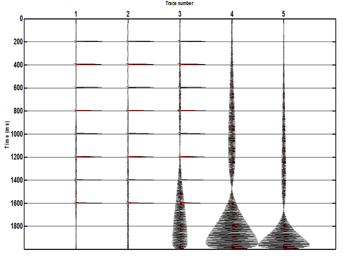  Figure 1. Inverse Qfiltered traces Q1=400,Q2=200,Q3=100,Q4=50,Q5=25

Low-passfiltering and inverse Q-filtering

In practice, the artefacts caused by numerical instability can be suppressed by a low-pass filter. Hale wrote that the unclipped IQF of a seismogram amplified the Nyquist frequency by a factor 7x10⁶ when we had the ratio t/Q=10 and concluded that for typical seismograms with lengths longer than 1000 samples and Q value around 100, data is seldom pure enough to warrant the use of unclipped IQF. Wang introduced a cutoff frequency to set up a criterion for the stabilization by a mathematical formula. However, considering Hales’ article it could be sufficient to simply remove the Nyquist frequency. That means to let the frequency close to Nyquist frequency be the cutoff frequency. On fig.2 we see a seismic model giving us benchmark data for inverse Q-filtering (red graph). We will see that IQF of this model will amplify the Nyquist frequency by a factor little less than 5x10⁶.

• 

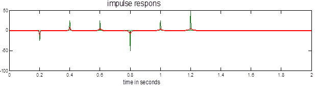  Figure 2. Seismic benchmark data model. Green graph is undamped and red graph is damped impulse response Q=50

Figure 3 is the amplitude-only inverse Q filtered trace of figure 2 for Q=50 (trace 4). The result clearly indicates the numerical instability. Artefacts are seen through the whole trace.

• 

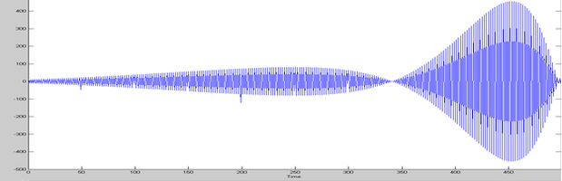  Fig.3. Model from fig.2. with applied invers Q-filter Q=50.

We will try to remove the artefacts by applying a low-pass filter on the trace of figure 3. We used MATLABS signal processing tool and created a low-passfilter (Zero-phase IIR-filter) on fig.4 with cutoff frequency at 120 Hz. The amplitude response of the filter is in blue and the phase in green.

• 

  Fig.4. Low-pass filter

The result of filtering trace on fig.3 with the low-passfilter of fig.4 is shown on fig.5. All artefacts are removed and we are left with the impulse response that can be compared with the original model on fig.2.

• 

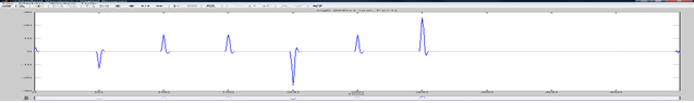  Figure 5. Filtered impulserespons where all unstable energy are removed.

Frequency-response

A study of the frequency response of the trace of figure 3 (unclipped) and figure 5 (clipped) will give more insight into the filtering process. Figure 6 shows the magnitude of the frequency response as a function of digital frequency before filtering. This representation gives a good picture of what happens around the Nyquist frequency when filtering with the low-pass filter is done. Unstable energy is accumulated close to the Nyquistfrequency. After filtering the unstable energy around the Nyquist-frequency is completely removed, and fig.7 give the frequency response of the impulse response of fig.5.

• 

  Figure 6. Frequency-response with digital frequency before filtering.

• 

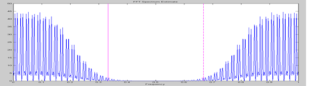  Figure 7. Frequency-response with digital frequency after filtering.

References

• Wang, Yanghua (2008). Seismic inverse Q filtering. Blackwell Pub.. ISBN 978-1-4051-8540-0. https://books.google.com/books?id=IpwAjT-F_TgC. 

External links

• Stabilized inverse Q filtering by Knut Sørsdal