Expected value of sample information

In decision theory, the expected value of sample information (EVSI) is the expected increase in utility that a decision-maker could obtain from gaining access to a sample of additional observations before making a decision. The additional information obtained from the sample may allow them to make a more informed, and thus better, decision, thus resulting in an increase in expected utility. EVSI attempts to estimate what this improvement would be before seeing actual sample data; hence, EVSI is a form of what is known as preposterior analysis. The use of EVSI in decision theory was popularized by Robert Schlaifer and Howard Raiffa in the 1960s.

Formulation

Let

[math]\displaystyle{ \begin{array}{ll} d\in D & \mbox{the decision being made, chosen from space } D \\ x\in X & \mbox{an uncertain state, with true value in space } X \\ z \in Z & \mbox{an observed sample composed of } n \mbox{ observations } \langle z_1,z_2,..,z_n \rangle \\ U(d,x) & \mbox{the utility of selecting decision } d \mbox{ from } x \\ p(x) & \mbox{the prior subjective probability distribution (density function) on } x \\ p(z|x) & \mbox{the conditional prior probability of observing the sample } z \end{array} }[/math]

It is common (but not essential) in EVSI scenarios for [math]\displaystyle{ Z_i=X }[/math], [math]\displaystyle{ p(z|x)=\prod p(z_i|x) }[/math] and [math]\displaystyle{ \int z p(z|x) dz = x }[/math], which is to say that each observation is an unbiased sensor reading of the underlying state [math]\displaystyle{ x }[/math], with each sensor reading being independent and identically distributed.

The utility from the optimal decision based only on the prior, without making any further observations, is given by

[math]\displaystyle{ E[U] = \max_{d\in D} ~ \int_X U(d,x) p(x) ~ dx. }[/math]

If the decision-maker could gain access to a single sample, [math]\displaystyle{ z }[/math], the optimal posterior utility would be

[math]\displaystyle{ E[U|z] = \max_{d\in D} ~ \int_X U(d,x) p(x|z) ~ dx }[/math]

where [math]\displaystyle{ p(x|z) }[/math] is obtained from Bayes' rule:

[math]\displaystyle{ }[/math]

[math]\displaystyle{ p(z) = \int p(z|x) p(x) ~ dx. }[/math]

Since they don't know what sample would actually be obtained if one were obtained, they must average over all possible samples to obtain the expected utility given a sample:

[math]\displaystyle{ E[U|SI] = \int_Z E[U|z] p(z) dz = \int_Z \max_{d\in D} ~ \int_X U(d,x) p(z|x) p(x) ~ dx ~ dz. }[/math]

The expected value of sample information is then defined as

[math]\displaystyle{ \begin{array}{rl} EVSI & = E[U|SI] - E[U] \\ & = \left(\int_Z \max_{d\in D} ~ \int_X U(d,x) p(z|x) p(x) ~ dx ~ dz\right) - \left(\max_{d\in D} ~ \int_X U(d,x) p(x) ~ dx\right). \end{array} }[/math]

Computation

It is seldom feasible to carry out the integration over the space of possible observations in E[U|SI] analytically, so the computation of EVSI usually requires a Monte Carlo simulation. The method involves randomly simulating a sample, [math]\displaystyle{ z^i=\langle z^i_1,z^i_2,..,z^i_n\rangle }[/math], then using it to compute the posterior [math]\displaystyle{ p(x|z^i) }[/math] and maximizing utility based on [math]\displaystyle{ p(x|z^i) }[/math]. This whole process is then repeated many times, for [math]\displaystyle{ i=1,..,M }[/math] to obtain a Monte Carlo sample of optimal utilities. These are averaged to obtain the expected utility given a hypothetical sample.

Example

A regulatory agency is to decide whether to approve a new treatment. Before making the final approve/reject decision, they ask what the value would be of conducting a further trial study on [math]\displaystyle{ n }[/math] subjects. This question is answered by the EVSI.

diagram of EVSI model

The diagram shows an influence diagram for computing the EVSI in this example.

The model classifies the outcome for any given subject into one of five categories:

[math]\displaystyle{ Z_i = }[/math] {"Cure", "Improvement", "Ineffective", "Mild side-effect", "Serious side-effect"}

And for each of these outcomes, assigns a utility equal to an estimated patient-equivalent monetary value of the outcome.

A decision state, [math]\displaystyle{ x }[/math] in this example is a vector of five numbers between 0 and 1 that sum to 1, giving the proportion of future patients that will experience each of the five possible outcomes. For example, a state [math]\displaystyle{ x=[5\%,60\%,20\%,10\%,5\%] }[/math] denotes the case where 5% of patients are cured, 60% improve, 20% find the treatment ineffective, 10% experience mild side-effects and 5% experience dangerous side-effects.

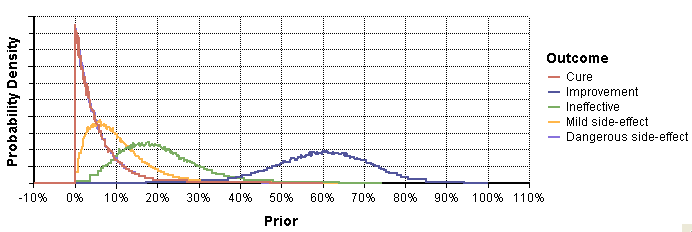
The prior, [math]\displaystyle{ p(x) }[/math] is encoded using a Dirichlet distribution, requiring five numbers (that don't sum to 1) whose relative values capture the expected relative proportion of each outcome, and whose sum encodes the strength of this prior belief. In the diagram, the parameters of the Dirichlet distribution are contained in the variable dirichlet alpha prior, while the prior distribution itself is in the chance variable Prior. The probability density graph of the marginals is shown here:

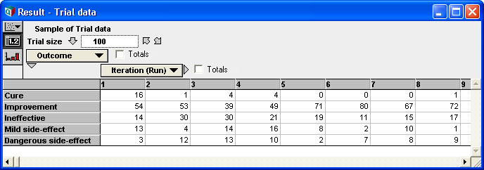
In the chance variable Trial data, trial data is simulated as a Monte Carlo sample from a Multinomial distribution. For example, when Trial_size=100, each Monte Carlo sample of Trial_data contains a vector that sums to 100 showing the number of subjects in the simulated study that experienced each of the five possible outcomes. The following result table depicts the first 8 simulated trial outcomes:

Combining this trial data with a Dirichlet prior requires only adding the outcome frequencies to the Dirichlet prior alpha values, resulting in a Dirichlet posterior distribution for each simulated trial. For each of these, the decision to approve is made based on whether the mean utility is positive, and using a utility of zero when the treatment is not approved, the Pre-posterior utility is obtained. Repeating the computation for a range of possible trial sizes, an EVSI is obtained at each possible candidate trial size as depicted in this graph:

Comparison to related measures

Expected value of sample information (EVSI) is a relaxation of the expected value of perfect information (EVPI) metric, which encodes the increase of utility that would be obtained if one were to learn the true underlying state, [math]\displaystyle{ x }[/math]. Essentially EVPI indicates the value of perfect information, while EVSI indicates the value of some limited and incomplete information.

The expected value of including uncertainty (EVIU) compares the value of modeling uncertain information as compared to modeling a situation without taking uncertainty into account. Since the impact of uncertainty on computed results is often analysed using Monte Carlo methods, EVIU appears to be very similar to the value of carrying out an analysis using a Monte Carlo sample, which closely resembles in statement the notion captured with EVSI. However, EVSI and EVIU are quite distinct—a notable difference between the manner in which EVSI uses Bayesian updating to incorporate the simulated sample.

See also

• Bayesian experimental design
• Expected value of perfect information (EVPI)
• Expected value of including uncertainty (EVIU)

Further reading

• Hamburg, Morris; Young, Peg (1993). "Devising Optimal Strategies Prior to Sampling". Statistical Analysis for Decision Making. Fort Worth: Dryden Press. pp. 731–766. ISBN 0-03-096914-X.