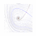
File:Hopf and homoclinic bifurcation 2.gif

From HandWiki

Original file(1,600 × 1,600 pixels, file size: 53.45 MB, MIME type: image/gif, 240 frames, 9.6 s)

Note: Due to technical limitations, thumbnails of high resolution GIF images such as this one will not be animated.

This file is from a shared repository and may be used by other projects. The description on its file description page there is shown below.

Summary

Description
English: ```python

from tqdm import tqdm import numpy as np import matplotlib.pyplot as plt from scipy.integrate import solve_ivp import os

escape_size = 2.0 # If a trajectory is this distance away from 0, we assume it has escaped and stop simulating it. for i, mu in enumerate(tqdm(np.linspace(-0.18, 0.15, 240))):

 if i < 129:
   continue
 def system(t, y):
     v, w = y
     dv = mu * v + w - v**2
     dw = -v + mu * w + 2 * v**2
     dv *= (np.abs(v) < 2.0) * (np.abs(w) < 2.0)
     dw *= (np.abs(v) < 2.0) * (np.abs(w) < 2.0)
     return [dv, dw]
 def system_reversed(t, y):
     v, w = y
     dv = mu * v + w - v**2
     dw = -v + mu * w + 2 * v**2
     dv *= (np.abs(v) < 2.0) * (np.abs(w) < 2.0)
     dw *= (np.abs(v) < 2.0) * (np.abs(w) < 2.0)
     return [-dv, -dw]
 x_root = (mu**2+1)/(2+mu)
 y_root = -mu * x_root + x_root ** 2
 vmin, vmax, wmin, wmax = -1,1,-1,1
 # vmin,vmax,wmin,wmax= x_root-0.0005,x_root+0.0005, y_root-0.0005, y_root+0.0005
 t_span = np.array([0, 20])
 trajectory_resolution = 10
 epsilon = 0.01
 
 initial_conditions = [(x, y)  for x in np.linspace(vmin, vmax, trajectory_resolution) for y in np.linspace(wmin, wmax, trajectory_resolution)]
 initial_conditions += [(0 + dx, 0 + dy) for dx in np.linspace(-0.02, 0.02, 3) for dy in np.linspace(-0.02, 0.02, 3)]
 initial_conditions_2 = [(x_root + dx, y_root + dy) for dx in np.linspace(-epsilon, epsilon, 10) for dy in np.linspace(-epsilon, epsilon, 10)]
 sols = {}
 sols_2 = {}
 sols_reversed = {}
 sols_reversed_2 = {}
 for ic in initial_conditions:
     sols[ic] = solve_ivp(system, t_span, ic, dense_output=True, max_step=0.05)
     sols_reversed[ic] = solve_ivp(system_reversed, t_span, ic, dense_output=True, max_step=0.05)
 for ic in initial_conditions_2:
     sols_2[ic] = solve_ivp(system, 2*t_span, ic, dense_output=True, max_step=0.05)
     sols_reversed_2[ic] = solve_ivp(system_reversed, 2*t_span, ic, dense_output=True, max_step=0.05)
 vs = np.linspace(vmin, vmax, 200)
 v_axis = np.linspace(vmin, vmax, 20)
 w_axis = np.linspace(wmin, wmax, 20)
 v_values, w_values = np.meshgrid(v_axis, w_axis)
 dv, dw = system(0, [v_values, w_values])
 fig, ax = plt.subplots(figsize=(16,16))
 # ax.scatter(x_root, y_root)
 # integral curves
 for ic in initial_conditions:
   sol = sols[ic]
   ax.plot(sol.y[0], sol.y[1],alpha=0.4, linewidth=0.5, color='k')
   sol = sols_reversed[ic]
   ax.plot(sol.y[0], sol.y[1], alpha=0.4, linewidth=0.5, color='k')
 for ic in initial_conditions_2:
   sol = sols_2[ic]
   ax.plot(sol.y[0], sol.y[1],alpha=0.8, linewidth=0.5, color='r')
   sol = sols_reversed_2[ic]
   ax.plot(sol.y[0], sol.y[1], alpha=0.8, linewidth=0.5, color='b')
 # vector fields
 arrow_lengths = np.sqrt(dv**2 + dw**2)
 alpha_values = 1 - (arrow_lengths / np.max(arrow_lengths))**0.4
 ax.quiver(v_values, w_values, dv, dw, color='blue', linewidth=0.5, scale=25, alpha=alpha_values)
 # nullclines
 ax.plot(vs, vs**2-mu*vs,  color="green", alpha=0.2, label="x nullcline")
 if np.abs(mu) < 0.001:
   ax.axvline(0, wmin, wmax, color="red", alpha=0.2, label="y nullcline")
   ax.axvline(1/2, wmin, wmax, color="red", alpha=0.2, label="y nullcline")
 else:  
   ax.plot(vs, (vs-2*vs**2)/mu, color="red", alpha=0.2, label="y nullcline")
ax.set_title(f'Hopf Bifurcation Model\n$\mu={mu:.3f
})
 # ax.legend()
 ax.set_xlim(vmin, vmax)
 ax.set_ylim(wmin, wmax)
 ax.set_xticks([])
 ax.set_yticks([])
 dir_path = f"./hopf_2"
 if not os.path.exists(dir_path):
   os.makedirs(dir_path)
 fig.savefig(f"{dir_path}/{i}.png")
 plt.close()

import imageio.v3 as iio from natsort import natsorted import moviepy.editor as mp

for dir_path in ["./hopf_2"]:

   file_names = natsorted((fn for fn in os.listdir(dir_path) if fn.endswith('.png')))
   # Create a list of image files and set the frame rate
   images = []
   fps = 24
   # Iterate over the file names and append the images to the list
   for file_name in file_names:
       file_path = os.path.join(dir_path, file_name)
       images.append(iio.imread(file_path))
   filename = dir_path[2:]
   iio.imwrite(f"{filename}.gif", images, duration=1000/fps, rewind=True)
   clip = mp.ImageSequenceClip(images, fps=fps)
   clip.write_videofile(f"{filename}.mp4")
```
Source Own work Edit this at Structured Data on Commons
Author

|date=2023-04-26 |source=Own work |author=Cosmia Nebula }}

Licensing

I, the copyright holder of this work, hereby publish it under the following license:
w:en:Creative Commons
attribution share alike
This file is licensed under the Creative Commons Attribution-Share Alike 4.0 International license.
You are free:
  • to share – to copy, distribute and transmit the work
  • to remix – to adapt the work
Under the following conditions:
  • attribution – You must give appropriate credit, provide a link to the license, and indicate if changes were made. You may do so in any reasonable manner, but not in any way that suggests the licensor endorses you or your use.
  • share alike – If you remix, transform, or build upon the material, you must distribute your contributions under the same or compatible license as the original.

Captions

Add a one-line explanation of what this file represents

Items portrayed in this file

depicts

image/gif

File history

Click on a date/time to view the file as it appeared at that time.

Date/TimeThumbnailDimensionsUserComment
current14:08, 26 April 2023Thumbnail for version as of 14:08, 26 April 20231,600 × 1,600 (53.45 MB)imagescommonswiki>Cosmia NebulaUploaded while editing "Bifurcation theory" on en.wikipedia.org

The following file is a duplicate of this file (more details):

The following 2 pages use this file: