Hopf bifurcation

In the mathematics of dynamical systems and differential equations, a Hopf bifurcation is said to occur when varying a parameter of the system causes the set of solutions (trajectories) to change from being attracted to (or repelled by) a fixed point, and instead become attracted to (or repelled by) an oscillatory, periodic solution.[1] The Hopf bifurcation is a two-dimensional analog of the pitchfork bifurcation.
Many different kinds of systems exhibit Hopf bifurcations, from radio oscillators to railroad bogies.[2] Trailers towed behind automobiles become infamously unstable if loaded incorrectly, or if designed with the wrong geometry. This offers an intuitive example of a Hopf bifurcation in the ordinary world, where stable motion becomes unstable and oscillatory as a parameter is varied. Fluid flows also exhibit Hopf bifurcation behavior when the transition from steady to unsteady laminar flow occurs.[3]
The general theory of how the solution sets of dynamical systems change in response to changes of parameters is called bifurcation theory; the term bifurcation arises, as the set of solutions typically split into several classes. Stability theory pursues the general theory of stability in mechanical, electronic and biological systems.
The conventional approach to locating Hopf bifurcations is to work with the Jacobian matrix associated with the system of differential equations. When this matrix has a pair of complex-conjugate eigenvalues that cross the imaginary axis as a parameter is varied, that point is the bifurcation. That crossing is associated with a stable fixed point "bifurcating" into a limit cycle.
A Hopf bifurcation is also known as a Poincaré–Andronov–Hopf bifurcation, named after Henri Poincaré, Aleksandr Andronov and Eberhard Hopf.
Overview
Hopf bifurcations occur in a large variety of dynamical systems described by differential equations. Near such a bifurcation, a two-dimensional subset of the dynamical system is approximated by a normal form, canonically expressed as the following time-dependent differential equation:
Here is the dynamical variable; it is a complex number. The parameter is real, and is a complex parameter. The number is called the first Lyapunov coefficient. The above has a simple exact solution, given below. This solution exhibits two distinct behaviors, depending on whether or . This change of behavior, as a function of is termed the "Hopf bifurcation".
The study of Hopf bifurcations is not so much the study of the above and its solution, as it is the study of how such two-dimensional subspaces can be identified and mapped onto this normal form. One approach is to examine the eigenvalues of the Jacobian matrix of the differential equations as a parameter is varied near the bifurcation point.
Exact solution

The normal form is effectively the Stuart–Landau equation, written with a different parameterization. It has a simple exact solution in polar coordinates. Writing and considering the real and imaginary parts as distinct, one obtains a pair of ordinary differential equations: and The second equation can be solved by observing that it is linear in . That is, which is just the shifted exponential equation. Re-arranging gives the generic solution
Depending on the sign of and , the trajectory of a point can be seen to spiral in to the origin, spiral out to infinity, or to approach a limit cycle.
Supercritical and subcritical Hopf bifurcations

The limit cycle is orbitally stable if the first Lyapunov coefficient is negative, and if Then the bifurcation is said to be supercritical. Otherwise it is unstable and the bifurcation is subcritical.
If is negative then there is a stable limit cycle for where This is the supercritical regime.
If is positive then there is an unstable limit cycle for The bifurcation is said to be subcritical. This classification into sub and super-critical bifurcations is analogous to that of the pitchfork bifurcation.
Jacobian
The Hopf bifurcation can be understood by examining the eigenvalues of the Jacobian matrix for the normal form. This is most readily done by re-writing the normal form in Cartesian coordinates . It then has the form where the shorthand and is used. The Jacobian is This is a bit tedious to compute: The fixed point was previously identified to be located at , at which location the Jacobian takes the particularly simple form: The corresponding characteristic polynomial is which has solutions Here, is a pair of complex conjugate eigenvalues of the Jacobian. When the parameter is negative, the real part of the eigenvalues is (obviously) negative. As the parameter crosses zero, the real part vanishes: this is the Hopf bifurcation. As previously seen, the limit cycle arises as goes positive if .
All Hopf bifurcations have this general form: the Jacobian matrix has a pair of complex-conjugate eigenvalues that cross the imaginary axis as the pertinent parameter is varied.
Linearization
The above computation of the Jacobian can be significantly simplified by working in the tangent plane, tangent to the fixed point. The fixed point is located at and so one can "linearize" the differential equation by dropping all terms that are higher than linear order. This gives
The Jacobian is computed exactly as before; nothing has changed, except to make the calculations simpler. The linearized differential equation can be recognized as being given by a Lie derivative defined on the tangent bundle. Because all cotangent bundles are always symplectic manifolds, it is common to formulate bifurcation theory in terms of symplectic geometry.[5]
Examples

Hopf bifurcations occur in the Lotka–Volterra model of predator–prey interaction (known as paradox of enrichment), the Hodgkin–Huxley model for nerve membrane potential,[6] the Selkov model of glycolysis,[7] the Belousov–Zhabotinsky reaction, the Lorenz attractor, the Brusselator, the delay differential equation and in classical electromagnetism.[8] Hopf bifurcations have also been shown to occur in fission waves.[9]
The Selkov model is
The figure shows a phase portrait illustrating the Hopf bifurcation in the Selkov model.[10]
In railway vehicle systems, Hopf bifurcation analysis is notably important. Conventionally a railway vehicle's stable motion at low speeds crosses over to unstable at high speeds. One aim of the nonlinear analysis of these systems is to perform an analytical investigation of bifurcation, nonlinear lateral stability and hunting behavior of rail vehicles on a tangent track, which uses the Bogoliubov method.[2]
Geometric interpretation
The benefit of the abstract formulation in terms of symplectic geometry is that it enables a geometric intuition into what otherwise seem to be complicated dynamical systems.
Consider the space of all possible solutions (point trajectories) to some set of differential equations. The tangent vectors to these solutions lie in the phase space for that system; more formally, in the tangent bundle. The phase space can be divided into three parts: the stable manifold, the unstable manifold, and the center manifold. The stable manifold consists of all of the tangent vector fields that, upon integration, approach the limit point or limit cycle. The unstable manifold consist of those vector fields that point away from the limit-point/limit cycle. The center manifold consists of the points on the limit, together with their tangent vectors.
The Hopf bifurcation is a rearrangement of these manifolds, as parameters are varied. For the normal form, the phase space is four-dimensional: the two coordinates and the two velocities When (and ) the entire (four-dimensional) space of solutions belongs to the stable manifold. As is varied, the center manifold changes from a point to a circle. As is varied, the stable manifold flips to become unstable.
In a general setting, the abstraction allows a four-dimensional subspace to be isolated from the full system, and then, as parameters are varied, all changes to the overall geometry are isolated to that four-dimensional subspace.
Formal definition of a Hopf bifurcation
The appearance or the disappearance of a periodic orbit through a local change in the stability properties of a fixed point is known as the Hopf bifurcation. The following theorem works for fixed points with one pair of conjugate nonzero purely imaginary eigenvalues. It tells the conditions under which this bifurcation phenomenon occurs.
Theorem (see section 11.2 of [11]). Let be the Jacobian of a continuous parametric dynamical system evaluated at a fixed point. Suppose that all eigenvalues of have negative real part except for one conjugate pair, varying as for some function of the parameters. A Hopf bifurcation arises when this eigenvalue pair cross the imaginary axis. This occurs as changes from negative to positive as the system parameters are varied.
Routh–Hurwitz criterion
The Routh–Hurwitz criterion (section I.13 of [12]) gives necessary conditions for a Hopf bifurcation to occur.[13]
Sturm series
Let be Sturm series associated to a characteristic polynomial . They can be written in the form: The coefficients for in correspond to what is called Hurwitz determinants.[13] Their definition is related to the associated Hurwitz matrix.
Propositions
Proposition 1. If all the Hurwitz determinants are positive, apart perhaps then the associated Jacobian has no pure imaginary eigenvalues.
Proposition 2. If all Hurwitz determinants (for all in are positive, and then all the eigenvalues of the associated Jacobian have negative real parts except a purely imaginary conjugate pair.
The conditions that we are looking for so that a Hopf bifurcation occurs (see theorem above) for a parametric continuous dynamical system are given by this last proposition.
Example
Consider the classical Van der Pol oscillator written with ordinary differential equations:
The Jacobian matrix associated to this system is
The characteristic polynomial (in ) of the Jacobian at the fixed point is The associated Sturm series is with coefficients
The Sturm polynomials can be written as (here ): For the Van der Pol oscillator, the coefficients are
A Hopf bifurcation can occur when proposition 2 is satisfied; in the present case, proposition 2 requires that
Clearly, the first and third conditions are satisfied; the second condition states that a Hopf bifurcation occurs for the Van der Pol oscillator when .
Serial expansion method
The serial expansion method provides a way for obtaining explicit solutions containing a Hopf bifurcation by means of a perturbative expansion in the order parameter.[14]
Consider a system defined by , where is smooth and is a parameter. The parameter should be written so that as increases from below zero to above zero, the origin turns from a spiral sink to a spiral source. A linear transform of parameters may be needed to place the equation into this form. For , a perturbative expansion is performed using two-timing:
where is "slow-time" (thus "two-timing"), and are functions of . By an argument of harmonic balance (see [14] for details), one may use . Placing the perturbative expansion for into , and keeping terms up to the produces three ordinary differential equations in .
The first equation is of form , which is solved by The are "slowly varying" functions of . Inserting this into the second equation allows it to be solved for .
Then plugging the solutions for into the third equation, an equation of form is obtained, with the right-hand-side a sum of trigonometric terms. Of these terms, the "resonance term", the one containing must be set to zero. This is the same idea as in the Poincaré–Lindstedt method. This provides two ordinary differential equations for , allowing one to solve for the equilibrium value of , as well as its stability.
Example of serial expansion
Consider the system defined by
This system has an equilibrium point at origin. When increases from negative to positive, the origin turns from a stable spiral point to an unstable spiral point. Eliminating from the equations gives a single second-order differential equation
The perturbative expansion to be performed is with Expanding up to order results in
The first equation has the solution Here are respectively the "slow-varying amplitude" and "slow-varying phase" of the simple oscillation. The second equation has solution where are also slow-varying amplitude and phase. The and terms can be absorbed into and equivalently, can be set without loss of generality. To demonstrate this, the perturbative expansion is written as
Basic trigonometry allows the two cosines to be merged into one:
for some and But this has exactly the same form as Thus, the term can be eliminated by redefining to be and to be The solution to the second equation is thus
Plugging through the third equation gives
Eliminating the resonance term gives
where the prime denotes differentiation by the slow time The first equation shows that is a stable equilibrium. The Hopf bifurcation creates an attracting (rather than repelling) limit cycle.
Plugging in gives . The time coordinate can be shifted so that . The third equation becomes
giving a solution
Plugging in back to the expressions for gives
Plugging these back to yields the serial expansion of as well, up to order .
After writing the solution is
and
This provides a parametric equation for the limit cycle. This is plotted in the illustration on the right.
- Examples of bifurcations
-
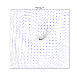 A Hopf bifurcation occurs in the system and , when , around the origin. A homoclinic bifurcation occurs around .
 -
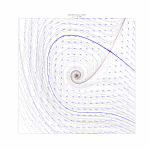 A detailed view of the homoclinic bifurcation.
 -
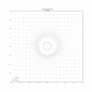 As increases from zero, a stable limit cycle emerges from the origin via Hopf bifurcation. The limit cycle is plotted parametrically, up to order .


See also
- Reaction–diffusion systems
References
- ↑ "Hopf Bifurcations.". MIT. https://ocw.mit.edu/courses/mathematics/18-385j-nonlinear-dynamics-and-chaos-fall-2004/lecture-notes/hopfbif.pdf.
- ↑ 2.0 2.1 Serajian, Reza (2011). "Effects of the bogie and body inertia on the nonlinear wheel-set hunting recognized by the hopf bifurcation theory". International Journal of Automotive Engineering 3 (4): 186–196. http://www.iust.ac.ir/ijae/article-1-25-en.pdf.
- ↑ Agnaou, M.; Lasseux, D.; Ahmadi, A. (2016). "From steady to unsteady laminar flow in model porous structures: an investigation of the first Hopf bifurcation". Computers & Fluids 136: 67–82. doi:10.1016/j.compfluid.2016.05.030. ISSN 0045-7930. https://www.sciencedirect.com/science/article/pii/S0045793016301797.
- ↑ Heitmann, S., Breakspear, M (2017-2022) Brain Dynamics Toolbox. bdtoolbox.org doi.org/10.5281/zenodo.5625923
- ↑ Abraham, R.; Marsden, J. E. (2008). Foundations of Mechanics: A Mathematical Exposition of Classical Mechanics with an Introduction to the Qualitative Theory of Dynamical Systems (2nd ed.). AMS Chelsea Publishing. ISBN 978-0-8218-4438-0.
- ↑ Guckenheimer, J.; Labouriau, J.S. (1993), "Bifurcation of the Hodgkin and Huxley equations: A new twist", Bulletin of Mathematical Biology 55 (5): 937–952, doi:10.1007/BF02460693.
- ↑ "Selkov Model Wolfram Demo". [demonstrations.wolfram.com ]. http://demonstrations.wolfram.com/HopfBifurcationInTheSelkovModel/.
- ↑ López, Álvaro G (2020-12-01). "Stability analysis of the uniform motion of electrodynamic bodies" (in en). Physica Scripta 96 (1): 015506. doi:10.1088/1402-4896/abcad2. ISSN 1402-4896.
- ↑ Osborne, Andrew G.; Deinert, Mark R. (October 2021). "Stability instability and Hopf bifurcation in fission waves" (in en). Cell Reports Physical Science 2 (10). doi:10.1016/j.xcrp.2021.100588. Bibcode: 2021CRPS....200588O.
- ↑ For detailed derivation, see Strogatz, Steven H. (1994). Nonlinear Dynamics and Chaos. Addison Wesley. p. 205. ISBN 978-0-7382-0453-6. https://archive.org/details/nonlineardynamic00stro/page/205.
- ↑ Hale, J.; Koçak, H. (1991). Dynamics and Bifurcations. Texts in Applied Mathematics. 3. Berlin: Springer-Verlag. ISBN 978-3-540-97141-2. https://archive.org/details/dynamicsbifurcat0000hale.
- ↑ Hairer, E.; Norsett, S. P.; Wanner, G. (1993). Solving Ordinary Differential Equations I: Nonstiff Problems (Second ed.). New York: Springer-Verlag. ISBN 978-3-540-56670-0.
- ↑ 13.0 13.1 Kahoui, M. E.; Weber, A. (2000). "Deciding Hopf bifurcations by quantifier elimination in a software component architecture". Journal of Symbolic Computation 30 (2): 161–179. doi:10.1006/jsco.1999.0353.
- ↑ 14.0 14.1 18.385J / 2.036J Nonlinear Dynamics and Chaos Fall 2014: Hopf Bifurcations. MIT OpenCourseWare
Further reading
- Guckenheimer, J.; Myers, M.; Sturmfels, B. (1997). "Computing Hopf Bifurcations I". SIAM Journal on Numerical Analysis 34 (1): 1–21. doi:10.1137/S0036142993253461.
- Hale, J.; Koçak, H. (1991). Dynamics and Bifurcations. Texts in Applied Mathematics. 3. Berlin: Springer-Verlag. ISBN 978-3-540-97141-2. https://archive.org/details/dynamicsbifurcat0000hale.
- Hassard, Brian D.; Kazarinoff, Nicholas D.; Wan, Yieh-Hei (1981). Theory and Applications of Hopf Bifurcation. New York: Cambridge University Press. ISBN 0-521-23158-2. https://books.google.com/books?id=3wU4AAAAIAAJ.
- Kuznetsov, Yuri A. (2004). Elements of Applied Bifurcation Theory (Third ed.). New York: Springer-Verlag. ISBN 978-0-387-21906-6.
- Strogatz, Steven H. (1994). Nonlinear Dynamics and Chaos. Addison Wesley. ISBN 978-0-7382-0453-6. https://archive.org/details/nonlineardynamic00stro.
External links
 |  |

