Gabor–Wigner transform

The Gabor transform, named after Dennis Gabor, and the Wigner distribution function, named after Eugene Wigner, are both tools for time-frequency analysis. Since the Gabor transform does not have high clarity, and the Wigner distribution function has a "cross term problem" (i.e. is non-linear), a 2007 study by S. C. Pei and J. J. Ding proposed a new combination of the two transforms that has high clarity and no cross term problem. Since the cross term does not appear in the Gabor transform, the time frequency distribution of the Gabor transform can be used as a filter to filter out the cross term in the output of the Wigner distribution function.

Mathematical definition

• Gabor transform

[math]\displaystyle{ G_x(t,f) = \int_{-\infty}^\infty e^{-\pi(\tau-t)^2}e^{-j2\pi f\tau}x(\tau) \, d\tau }[/math]

• Wigner distribution function

[math]\displaystyle{ W_x(t,f)=\int_{-\infty}^\infty x(t+\tau/2)x^*(t-\tau/2)e^{-j2\pi\tau\,f} \, d\tau }[/math]

• Gabor–Wigner transform

There are many different combinations to define the Gabor–Wigner transform. Here four different definitions are given.

1. [math]\displaystyle{ D_x(t,f)=G_x(t,f)\times W_x(t,f) }[/math]
2. [math]\displaystyle{ D_x(t,f)=\min\left\{|G_x(t,f)|^2,|W_x(t,f)|\right\} }[/math]
3. [math]\displaystyle{ D_x(t,f)=W_x(t,f)\times \{|G_x(t,f)|\gt 0.25\} }[/math]
4. [math]\displaystyle{ D_x(t,f)=G_x^{2.6}(t,f)W_x^{0.7}(t,f) }[/math]

Character

1. Cross Term Problem:

   The definition of Wigner distribution function (WDF) is [math]\displaystyle{ W_x(t,f) = \int^{\infty}_{-\infty}x(t+\frac{\tau}{2})x^*(t-\frac{\tau}{2})e^{-j2\pi \tau f} \cdot d\tau }[/math]

   [math]\displaystyle{ x }[/math] is the input signal, [math]\displaystyle{ t }[/math] the time axis after transform, [math]\displaystyle{ f }[/math] is the frequency axis after transform.

   If we design our input signal as : [math]\displaystyle{ x(t) = \alpha g(t) + \beta s(t) }[/math], and its WDF presents as below:

   [math]\displaystyle{ \begin{align} W_x(t,f) &= \int^{\infty}_{-\infty}x(t+\frac{\tau}{2})x^*(t-\frac{\tau}{2})e^{-j2\pi \tau f} \cdot d\tau \\ &= \int^{\infty}_{-\infty} \big[ \alpha g(t+\frac{\tau}{2}) + \beta s(t+\frac{\tau}{2}) \big] \big[ \alpha^* g^*(t-\frac{\tau}{2}) + \beta^* s^*(t-\frac{\tau}{2}) \big]e^{-j2\pi \tau f} \cdot d\tau \\ &= \int^{\infty}_{-\infty} \big[ |\alpha|^2 g(t+\frac{\tau}{2})g^*(t-\frac{\tau}{2}) + |\beta|^2 s(t+\frac{\tau}{2})s^*(t-\frac{\tau}{2}) \\ &\quad + \alpha \beta^* g(t+\frac{\tau}{2})s^*(t-\frac{\tau}{2}) + \alpha^* \beta g^*(t-\frac{\tau}{2})s(t+\frac{\tau}{2}) \big] e^{-j2\pi \tau f} \cdot d\tau \\ &= |\alpha|^2 W_g(t,f)+|\beta|^2W_s(t,f) \\ &\quad + \int^{\infty}_{-\infty} \big[ \alpha \beta^* g(t+\frac{\tau}{2})s^*(t-\frac{\tau}{2}) + \alpha^* \beta g^*(t-\frac{\tau}{2})s(t+\frac{\tau}{2}) \big] e^{-j2\pi \tau f} \cdot d\tau \\ \end{align} }[/math]

   [math]\displaystyle{ W_g }[/math] and [math]\displaystyle{ W_s }[/math] are called "auto-term", and other components are "cross-term", which is not the correct information from the original signal.

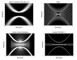
   The Gabor Transform (GT) can avoid the cross-term problem, while the Wigner-distribution function (WDF) has high clarity. By combining the two, the Gabor-Wigner Transform (GWT) achieves both high clarity and the ability to avoid the cross-term problem. Example are shown in the picture below.

   

   時頻分析2

2. Rotation relation:

   The GWT has rotation relation with the FRFT, making it useful for filter design, sampling, and multiplexing in the FRFT domain.

Application

The Gabor-Wigner transform performs well in image processing, filter design, signal sampling, modulation, demodulation, speech processing, and biomedical engineering.

Filter Design

The goal of filter design is to remove unwanted portions of the signal while preserving the necessary parts. By using the Gabor-Wigner transform, we can simultaneously consider filters in both the time domain and frequency domain, representing a form of time-frequency analysis. The main concept is illustrated as follows.

Filter fractional

Signal Modulation

The purpose of modulation is to place a signal within a specific time or frequency range. Using the Gabor-Wigner transform, we can simultaneously consider how to introduce more or more suitable signal patterns in both the time and frequency domains. Due to the absence of cross-term issues, it performs better than the Wigner transform.

Mul mod

From the figure (WDF) above, it can also be observed that when using the Wigner transform (WDF), the generated cross-terms have a severe impact on modulation.

Technique for fast implementation of the Gabor-Wigner Transform

1. Due to the lower complexity of the Gabor transform compared to the Wigner transform, the Gabor transform is usually prioritized for calculation. When calculating the Wigner transform, it is only necessary to compute the Gabor transform in non-zero regions, as the values in other regions approach zero. Mathematically, this can be expressed as

   [math]\displaystyle{ G_X(t,f)\approx 0, D_x(t,f) = G_x^\alpha(t,f)W_x^\beta(t,f) \approx 0 }[/math]

2. When [math]\displaystyle{ x(t) }[/math] is a real function, for the Gabor transform, [math]\displaystyle{ X(f) = X^*(-f) }[/math]. This allows for a significant reduction in the required memory area when designing memory.

Comparison

Time-frequency analysis	Advantages	Disadvantages	Complexity
Gabor transform	without cross-term	lower clarity	Low
Wigner-distirbution function	higher clarity	with cross-term	Medium
Gabor-Wigner transform	high clarity and without cross-term	high computational load	High

See also

• Time-frequency representation
• Short-time Fourier transform
• Gabor transform
• Wigner distribution function

References

- ↑ S. C. Pei and J. J. Ding, “Relations between Gabor transforms and fractional Fourier transforms and their applications for signal processing,” IEEE Trans. Signal Process., vol. 55, no. 10, pp. 4839–4850, Oct. 2007.