Gegenbauer polynomials

Short description: Polynomial sequence

In mathematics, Gegenbauer polynomials or ultraspherical polynomials C(α)n(x) are orthogonal polynomials on the interval [−1,1] with respect to the weight function (1 − x²)^α–1/2. They generalize Legendre polynomials and Chebyshev polynomials, and are special cases of Jacobi polynomials. They are named after Leopold Gegenbauer.

Characterizations

• 
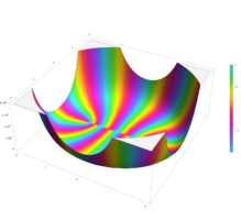  Plot of the Gegenbauer polynomial C n^(m)(x) with n=10 and m=1 in the complex plane from -2-2i to 2+2i with colors created with Mathematica 13.1 function ComplexPlot3D
• 
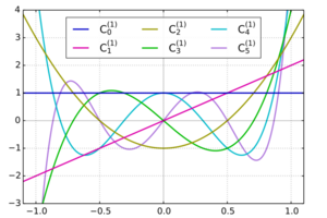  Gegenbauer polynomials with α=1
• 
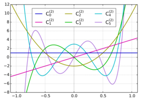  Gegenbauer polynomials with α=2
• 
  Gegenbauer polynomials with α=3
• 
  An animation showing the polynomials on the xα-plane for the first 4 values of n.

A variety of characterizations of the Gegenbauer polynomials are available.

• The polynomials can be defined in terms of their generating function (Stein Weiss):

$\frac{1}{(1-2xt+t^2{)}^{\alpha }}=\sum _{n=0}^{\mathrm{\infty }}{C}_n^{(\alpha )}(x)t^n(0\le |x|<1,|t|\le 1,\alpha >0)$

• The polynomials satisfy the recurrence relation (Suetin 2001):

$\begin{array}{rl}{C}_0^{(\alpha )}(x)& =1\\ C_1^{(\alpha )}(x)& =2\alpha x\\ (n+1)C_{n+1}^{(\alpha )}(x)& =2(n+\alpha )x{C}_n^{(\alpha )}(x)-(n+2\alpha -1)C_{n-1}^{(\alpha )}(x).\end{array}$

• Gegenbauer polynomials are particular solutions of the Gegenbauer differential equation (Suetin 2001):

$(1-x^2)y^{″}-(2\alpha +1)x{y}^{\prime }+n(n+2\alpha )y=0.$

When α = 1/2, the equation reduces to the Legendre equation, and the Gegenbauer polynomials reduce to the Legendre polynomials.

When α = 1, the equation reduces to the Chebyshev differential equation, and the Gegenbauer polynomials reduce to the Chebyshev polynomials of the second kind.

• They are given as Gaussian hypergeometric series in certain cases where the series is in fact finite:

$C_n^{(\alpha )}(z)=\frac{(2\alpha {)}_n}{n!}{}_2{F}_1(-n,2\alpha +n;\alpha +\frac{1}{2};\frac{1-z}{2}).$

(Abramowitz & Stegun p. 561). Here (2α)_n is the rising factorial. Explicitly,

$C_n^{(\alpha )}(z)=\sum _{k=0}^{\lfloor n/2\rfloor }(-1{)}^k\frac{\mathrm{\Gamma }(n-k+\alpha )}{\mathrm{\Gamma }(\alpha )k!(n-2k)!}(2z{)}^{n-2k}.$

From this it is also easy to obtain the value at unit argument:

$C_n^{(\alpha )}(1)=\frac{\mathrm{\Gamma }(2\alpha +n)}{\mathrm{\Gamma }(2\alpha )n!}.$

• They are special cases of the Jacobi polynomials (Suetin 2001):

$C_n^{(\alpha )}(x)=\frac{(2\alpha {)}_n}{(\alpha +\frac{1}{2}{)}_n}{P}_n^{(\alpha -1/2,\alpha -1/2)}(x).$

in which $(\theta {)}_n$ represents the rising factorial of $\theta$.

One therefore also has the Rodrigues formula

$C_n^{(\alpha )}(x)=\frac{(-1{)}^n}{2^{n}n!}\frac{\mathrm{\Gamma }(\alpha +\frac{1}{2})\mathrm{\Gamma }(n+2\alpha )}{\mathrm{\Gamma }(2\alpha )\mathrm{\Gamma }(\alpha +n+\frac{1}{2})}(1-x^2{)}^{-\alpha +1/2}\frac{d^n}{d{x}^n}[(1-x^2{)}^{n+\alpha -1/2}].$

• An alternative normalization sets $C_n^{(\alpha )}(1)=1$. Assuming this alternative normalization, the derivatives of Gegenbauer are expressed in terms of Gegenbauer:

$$\begin{array}{rl}\frac{d^q}{d{x}^q}{C}_{q+2j+1}^{(\alpha )}(x)=\frac{2^q(q+2j+1)!}{(q-1)!\mathrm{\Gamma }(q+2j+2\alpha +1)}& \sum _{i=0}^j\frac{(2i+\alpha +1)\mathrm{\Gamma }(2i+2\alpha +1)}{(2i+1)!(j-i)!}\\ & \times \frac{\mathrm{\Gamma }(q+j+i+\alpha +1)}{\mathrm{\Gamma }(j+i+\alpha +2)}(q+j-i-1)!C_{2i+1}^{(\alpha )}(x)\end{array}$$

Orthogonality and normalization

For a fixed α > -1/2, the polynomials are orthogonal on [−1, 1] with respect to the weighting function (Abramowitz & Stegun p. 774)

$w(z)={(1-z^2)}^{\alpha -\frac{1}{2}}.$

To wit, for n ≠ m,

$\underset{-1}{\overset{1}{\int }}{C}_n^{(\alpha )}(x)C_m^{(\alpha )}(x)(1-x^2{)}^{\alpha -\frac{1}{2}}dx=0.$

They are normalized by

$\underset{-1}{\overset{1}{\int }}{[C_n^{(\alpha )}(x)]}^2(1-x^2{)}^{\alpha -\frac{1}{2}}dx=\frac{\pi 2^{1-2\alpha }\mathrm{\Gamma }(n+2\alpha )}{n!(n+\alpha )[\mathrm{\Gamma }(\alpha ){]}^2}.$

Applications

The Gegenbauer polynomials appear naturally as extensions of Legendre polynomials in the context of potential theory and harmonic analysis. The Newtonian potential in Rⁿ has the expansion, valid with α = (n − 2)/2,

$\frac{1}{|\mathbf{𝐱}-\mathbf{𝐲}{|}^{n-2}}=\sum _{k=0}^{\mathrm{\infty }}\frac{|\mathbf{𝐱}{|}^k}{|\mathbf{𝐲}{|}^{k+n-2}}{C}_k^{(\alpha )}(\frac{\mathbf{𝐱}\cdot \mathbf{𝐲}}{|\mathbf{𝐱}||\mathbf{𝐲}|}).$

When n = 3, this gives the Legendre polynomial expansion of the gravitational potential. Similar expressions are available for the expansion of the Poisson kernel in a ball (Stein Weiss).

It follows that the quantities $C_k^{((n-2)/2)}(\mathbf{𝐱}\cdot \mathbf{𝐲})$ are spherical harmonics, when regarded as a function of x only. They are, in fact, exactly the zonal spherical harmonics, up to a normalizing constant.

Gegenbauer polynomials also appear in the theory of positive-definite functions.

The Askey–Gasper inequality reads

$\sum _{j=0}^n\frac{C_j^{\alpha }(x)}{(\genfrac{}{}{0ex}{}{2\alpha +j-1}{j})}\ge 0(x\ge -1,\alpha \ge 1/4).$

In spectral methods for solving differential equations, if a function is expanded in the basis of Chebyshev polynomials and its derivative is represented in a Gegenbauer/ultraspherical basis, then the derivative operator becomes a diagonal matrix, leading to fast banded matrix methods for large problems.

Other properties

Dirichlet–Mehler-type integral representation:$$\frac{P_n^{(\alpha ,\alpha )}(\cos \theta )}{P_n^{(\alpha ,\alpha )}\left(1\right)}=\frac{C_n^{(\alpha +\frac{1}{2})}(\cos \theta )}{C_n^{(\alpha +\frac{1}{2})}\left(1\right)}=\frac{2^{\alpha +\frac{1}{2}}\mathrm{\Gamma }(\alpha +1)}{{\pi }^{\frac{1}{2}}\mathrm{\Gamma }(\alpha +\frac{1}{2})}(\sin \theta {)}^{-2\alpha }\underset{0}{\overset{\theta }{\int }}\frac{\cos ((n+\alpha +\frac{1}{2})\varphi )}{(\cos \varphi -\cos \theta {)}^{-\alpha +\frac{1}{2}}}\mathrm{d}\varphi ,$$Laplace-type integral representation$$\begin{array}{rl}\frac{P_n^{(\alpha ,\alpha )}(\cos \theta )}{P_n^{(\alpha ,\alpha )}(1)}& =\frac{C_n^{(\alpha +\frac{1}{2})}(\cos \theta )}{C_n^{(\alpha +\frac{1}{2})}(1)}\\ & =\frac{\mathrm{\Gamma }(\alpha +1)}{{\pi }^{\frac{1}{2}}\mathrm{\Gamma }(\alpha +\frac{1}{2})}\underset{0}{\overset{\pi }{\int }}(\cos \theta +i\sin \theta \cos \varphi {)}^n(\sin \varphi {)}^{2\alpha }\mathrm{d}\varphi \end{array}$$Addition formula:

$$\begin{array}{rl}& C_n^{\lambda }(\cos {\theta }_1\cos {\theta }_2+\sin {\theta }_1\sin {\theta }_2\cos \varphi )\\ & =\sum _{k=0}^n{a}_{n,k}^{\lambda }{(\sin {\theta }_1)}^k{C}_{n-k}^{\lambda +k}(\cos {\theta }_1){(\sin {\theta }_2)}^k{C}_{n-k}^{\lambda +k}(\cos {\theta }_2)\\ & \cdot C_k^{\lambda -1/2}(\cos \varphi ),a_{n,k}^{\lambda }\text{ constants }\end{array}$$

Asymptotics

Given fixed $\lambda \in (0,1),M\in \{1,2,\dots \},\delta \in (0,\pi /2)$, uniformly for all $\theta \in [\delta ,\pi -\delta ]$, for $n\to \mathrm{\infty }$,$$C_n^{(\lambda )}(\cos \theta )=\frac{2^{2\lambda }\mathrm{\Gamma }(\lambda +\frac{1}{2})}{{\pi }^{\frac{1}{2}}\mathrm{\Gamma }(\lambda +1)}\frac{{\left(2\lambda \right)}_n}{{(\lambda +1)}_n}(\sum _{m=0}^{M-1}\frac{{\left(\lambda \right)}_m{(1-\lambda )}_m}{m!{(n+\lambda +1)}_m}\frac{\cos {\theta }_{n,m}}{(2\sin \theta {)}^{m+\lambda }}+R_M(\theta ))$$

where $(\cdot {)}_m$ is the Pochhammer symbol, and$${\theta }_{n,m}=(n+m+\lambda )\theta -\frac{1}{2}(m+\lambda )\pi$$The remainder $R_M=O\left(\frac{1}{n^M}\right)$ has an explicit upper bound:$$|R_M(\theta )|\le (2/\pi )\sin (\lambda \pi )\frac{\mathrm{\Gamma }(n+2\lambda )}{\mathrm{\Gamma }(\lambda )}\frac{\mathrm{\Gamma }(M+\lambda )\mathrm{\Gamma }(M-\lambda +1)}{M!\mathrm{\Gamma }(n+M+\lambda +1)}\frac{\max (|\cos \theta {|}^{-1},2\sin \theta )}{(2\sin \theta {)}^{M+\lambda }}$$where $\mathrm{\Gamma }$ is the Gamma function.

Other asymptotic formulas can be obtained as special cases of asymptotic formulas for the more general Jacobi polynomials.

See also

• Rogers polynomials, the q-analogue of Gegenbauer polynomials
• Chebyshev polynomials
• Romanovski polynomials

References

• Abramowitz, Milton; Stegun, Irene Ann, eds (1983). "Chapter 22". Handbook of Mathematical Functions with Formulas, Graphs, and Mathematical Tables. Applied Mathematics Series. 55 (Ninth reprint with additional corrections of tenth original printing with corrections (December 1972); first ed.). Washington D.C.; New York: United States Department of Commerce, National Bureau of Standards; Dover Publications. pp. 773. LCCN 65-12253. ISBN 978-0-486-61272-0. http://www.math.sfu.ca/~cbm/aands/page_773.htm. *Koornwinder, Tom H.; Wong, Roderick S. C.; Koekoek, Roelof; Swarttouw, René F. (2010), "Orthogonal Polynomials", in Olver, Frank W. J.; Lozier, Daniel M.; Boisvert, Ronald F. et al., NIST Handbook of Mathematical Functions, Cambridge University Press, ISBN 978-0-521-19225-5, http://dlmf.nist.gov/18 
• Stein, Elias; Weiss, Guido (1971), Introduction to Fourier Analysis on Euclidean Spaces, Princeton, N.J.: Princeton University Press, ISBN 978-0-691-08078-9, https://archive.org/details/introductiontofo0000stei .
• Szegő, G. (1975). Orthogonal Polynomials. Colloquium Publications. XXIII (4th ed.). Providence, RI: American Mathematical Society. 
• Hazewinkel, Michiel, ed. (2001), "Ultraspherical polynomials", Encyclopedia of Mathematics, Springer Science+Business Media B.V. / Kluwer Academic Publishers, ISBN 978-1-55608-010-4, https://www.encyclopediaofmath.org/index.php?title=U/u095030 .

Specific