Homography (computer vision)

Short description: Relation of two images with software

Geometrical setup for homography: stereo cameras O₁ and O₂ both pointed at X in epipolar geometry. Drawing from Neue Konstruktionen der Perspektive und Photogrammetrie by Hermann Guido Hauck (1845 — 1905)

In the field of computer vision, any two images of the same planar surface in space are related by a homography (assuming a pinhole camera model). This has many practical applications, such as image rectification, image registration, or camera motion—rotation and translation—between two images. Once camera resectioning has been done from an estimated homography matrix, this information may be used for navigation, or to insert models of 3D objects into an image or video, so that they are rendered with the correct perspective and appear to have been part of the original scene (see Augmented reality).

3D plane to plane equation

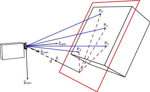
We have two cameras a and b, looking at points [math]\displaystyle{ P_i }[/math] in a plane. Passing from the projection [math]\displaystyle{ {}^bp_i=\left({}^bu_i;{}^bv_i;1\right) }[/math] of [math]\displaystyle{ P_i }[/math] in b to the projection [math]\displaystyle{ {}^ap_i=\left({}^au_i;{}^av_i;1\right) }[/math] of [math]\displaystyle{ P_i }[/math] in a:

[math]\displaystyle{ {}^ap_i = \frac{{}^bz_i}{{}^az_i}K_a \cdot H_{ab} \cdot K_b^{-1} \cdot {}^bp_i }[/math]

where [math]\displaystyle{ {}^az_i }[/math] and [math]\displaystyle{ {}^bz_i }[/math] are the z coordinates of P in each camera frame and where the homography matrix [math]\displaystyle{ H_{ab} }[/math] is given by

[math]\displaystyle{ H_{ab} = R - \frac{t n^T}{d} }[/math].

[math]\displaystyle{ R }[/math] is the rotation matrix by which b is rotated in relation to a; t is the translation vector from a to b; n and d are the normal vector of the plane and the distance from origin to the plane respectively. K_a and K_b are the cameras' intrinsic parameter matrices.

The figure shows camera b looking at the plane at distance d. Note: From above figure, assuming [math]\displaystyle{ n^T P_i + d = 0 }[/math] as plane model, [math]\displaystyle{ n^T P_i }[/math] is the projection of vector [math]\displaystyle{ P_i }[/math] along [math]\displaystyle{ n }[/math], and equal to [math]\displaystyle{ -d }[/math]. So [math]\displaystyle{ t = t \cdot 1 = t \left(-\frac{n^TP_i}{d}\right) }[/math]. And we have [math]\displaystyle{ H_{ab} P_i = R P_i + t }[/math] where [math]\displaystyle{ H_{ab} = R - \frac{t n^T}{d} }[/math].

This formula is only valid if camera b has no rotation and no translation. In the general case where [math]\displaystyle{ R_a,R_b }[/math] and [math]\displaystyle{ t_a,t_b }[/math] are the respective rotations and translations of camera a and b, [math]\displaystyle{ R=R_a R_b^T }[/math] and the homography matrix [math]\displaystyle{ H_{ab} }[/math] becomes

[math]\displaystyle{ H_{ab} = R_a R_b^T - \frac{(-R_a * R_b^T * t_b + t_a) n^T}{d} }[/math]

where d is the distance of the camera b to the plane.

Affine homography

When the image region in which the homography is computed is small or the image has been acquired with a large focal length, an affine homography is a more appropriate model of image displacements. An affine homography is a special type of a general homography whose last row is fixed to

[math]\displaystyle{ h_{31}=h_{32}=0, \; h_{33}=1. }[/math]

See also

• Direct linear transformation
• Epipolar geometry
• Feature (computer vision)
• Fundamental matrix (computer vision)
• Pose (computer vision)
• Photogrammetry

References

• O. Chum and T. Pajdla and P. Sturm (2005). "The Geometric Error for Homographies". Computer Vision and Image Understanding 97 (1): 86–102. doi:10.1016/j.cviu.2004.03.004. http://perception.inrialpes.fr/Publications/2005/CPS05/ChumPajdlaSturm-cviu05.pdf. 

Toolboxes

• homest is a GPL C/C++ library for robust, non-linear (based on the Levenberg–Marquardt algorithm) homography estimation from matched point pairs (Manolis Lourakis).
• OpenCV is a complete (open and free) computer vision software library that has many routines related to homography estimation (cvFindHomography) and re-projection (cvPerspectiveTransform).

External links

• Serge Belongie & David Kriegman (2007) Explanation of Homography Estimation from Department of Computer Science and Engineering, University of California, San Diego.
• A. Criminisi, I. Reid & A. Zisserman (1997) "A Plane Measuring Device", §3 Computing the Plane to Plane Homography, from Visual Geometry Group, Department of Engineering Science, University of Oxford.
• Elan Dubrofsky (2009) Homography Estimation, Master's thesis, from Department of Computer Science, University of British Columbia.
• Richard Hartley & Andrew Zisserman (2004) Multiple View Geometry from Visual Geometry Group, Oxford. Includes Matlab Functions for calculating a homography and the fundamental matrix (computer vision).
• GIMP Tutorial – using the Perspective Tool by Billy Kerr on YouTube. Shows how to do a perspective transform using GIMP.
• Allan Jepson (2010) Planar Homographies from Department of Computer Science, University of Toronto. Includes 2D homography from four pairs of corresponding points, mosaics in image processing, removing perspective distortion in computer vision, rendering textures in computer graphics, and computing planar shadows.
• Plane transfer homography Course notes from CSE576 at University of Washington in Seattle.
• Etienne Vincent & Robert Laganiere (2000) Detecting Planar Homographies in an Image Pair from School of Information Technology and Engineering, University of Ottawa. Describes an algorithm for detecting planes in images, uses random sample consensus (RANSAC) method, describes heuristics and iteration.