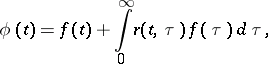
Integral equation of convolution type
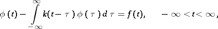
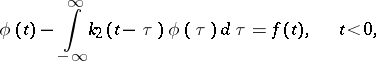
An integral equation containing the unknown function under the integral sign of a convolution transform (see Integral operator). The peculiarity of an integral equation of convolution type is that the kernel of such an equation depends on the difference of the arguments. The simplest example is the equation
| <img align="absmiddle" border="0" src="https://www.encyclopediaofmath.org/legacyimages/i/i051/i051410/i0514101.png" /> | (1) |
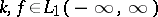
where <img align="absmiddle" border="0" src="https://www.encyclopediaofmath.org/legacyimages/i/i051/i051410/i0514102.png" /> and <img align="absmiddle" border="0" src="https://www.encyclopediaofmath.org/legacyimages/i/i051/i051410/i0514103.png" /> are given functions and <img align="absmiddle" border="0" src="https://www.encyclopediaofmath.org/legacyimages/i/i051/i051410/i0514104.png" /> is the unknown function. Suppose that <img align="absmiddle" border="0" src="https://www.encyclopediaofmath.org/legacyimages/i/i051/i051410/i0514105.png" /> and that one seeks a solution in the same class. In order that (1) is solvable it is necessary and sufficient that the following condition holds:
| <img align="absmiddle" border="0" src="https://www.encyclopediaofmath.org/legacyimages/i/i051/i051410/i0514106.png" /> | (2) |
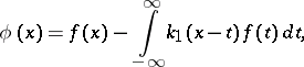
where <img align="absmiddle" border="0" src="https://www.encyclopediaofmath.org/legacyimages/i/i051/i051410/i0514107.png" /> is the Fourier transform of <img align="absmiddle" border="0" src="https://www.encyclopediaofmath.org/legacyimages/i/i051/i051410/i0514108.png" />. When (2) holds, equation (1) has a unique solution in the class <img align="absmiddle" border="0" src="https://www.encyclopediaofmath.org/legacyimages/i/i051/i051410/i0514109.png" />, representable by the formula
| <img align="absmiddle" border="0" src="https://www.encyclopediaofmath.org/legacyimages/i/i051/i051410/i05141010.png" /> | (3) |
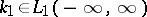
where <img align="absmiddle" border="0" src="https://www.encyclopediaofmath.org/legacyimages/i/i051/i051410/i05141011.png" /> is uniquely determined by its Fourier transform
| <img align="absmiddle" border="0" src="https://www.encyclopediaofmath.org/legacyimages/i/i051/i051410/i05141012.png" /> |
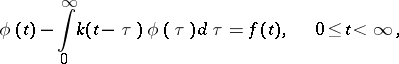
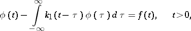
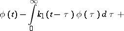
An equation of convolution type on the half-line (a Wiener–Hopf equation)
| <img align="absmiddle" border="0" src="https://www.encyclopediaofmath.org/legacyimages/i/i051/i051410/i05141013.png" /> | (4) |
arises in the study of various questions of theoretical and applied character (see [1], [4]).
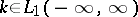
Suppose that the right-hand side <img align="absmiddle" border="0" src="https://www.encyclopediaofmath.org/legacyimages/i/i051/i051410/i05141014.png" /> and the unknown function <img align="absmiddle" border="0" src="https://www.encyclopediaofmath.org/legacyimages/i/i051/i051410/i05141015.png" /> belong to <img align="absmiddle" border="0" src="https://www.encyclopediaofmath.org/legacyimages/i/i051/i051410/i05141016.png" />, <img align="absmiddle" border="0" src="https://www.encyclopediaofmath.org/legacyimages/i/i051/i051410/i05141017.png" />, that the kernel <img align="absmiddle" border="0" src="https://www.encyclopediaofmath.org/legacyimages/i/i051/i051410/i05141018.png" /> and that
| <img align="absmiddle" border="0" src="https://www.encyclopediaofmath.org/legacyimages/i/i051/i051410/i05141019.png" /> | (5) |
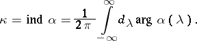
The function <img align="absmiddle" border="0" src="https://www.encyclopediaofmath.org/legacyimages/i/i051/i051410/i05141020.png" /> is called the symbol of equation (4). The index of equation (4) is the number
| <img align="absmiddle" border="0" src="https://www.encyclopediaofmath.org/legacyimages/i/i051/i051410/i05141021.png" /> | (6) |
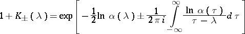
If <img align="absmiddle" border="0" src="https://www.encyclopediaofmath.org/legacyimages/i/i051/i051410/i05141022.png" />, then the functions <img align="absmiddle" border="0" src="https://www.encyclopediaofmath.org/legacyimages/i/i051/i051410/i05141023.png" /> defined by the equations
| <img align="absmiddle" border="0" src="https://www.encyclopediaofmath.org/legacyimages/i/i051/i051410/i05141024.png" /> | (7) |
are the Fourier transforms of functions <img align="absmiddle" border="0" src="https://www.encyclopediaofmath.org/legacyimages/i/i051/i051410/i05141025.png" />, respectively, such that <img align="absmiddle" border="0" src="https://www.encyclopediaofmath.org/legacyimages/i/i051/i051410/i05141026.png" /> for <img align="absmiddle" border="0" src="https://www.encyclopediaofmath.org/legacyimages/i/i051/i051410/i05141027.png" />. Under the above conditions, equation (4) has a unique solution, which can be expressed by the formula
| <img align="absmiddle" border="0" src="https://www.encyclopediaofmath.org/legacyimages/i/i051/i051410/i05141028.png" /> | (8) |
where
| <img align="absmiddle" border="0" src="https://www.encyclopediaofmath.org/legacyimages/i/i051/i051410/i05141029.png" /> |
If <img align="absmiddle" border="0" src="https://www.encyclopediaofmath.org/legacyimages/i/i051/i051410/i05141030.png" />, all solutions of equation (4) are given by the formula
| <img align="absmiddle" border="0" src="https://www.encyclopediaofmath.org/legacyimages/i/i051/i051410/i05141031.png" /> | (9) |
| <img align="absmiddle" border="0" src="https://www.encyclopediaofmath.org/legacyimages/i/i051/i051410/i05141032.png" /> |
where <img align="absmiddle" border="0" src="https://www.encyclopediaofmath.org/legacyimages/i/i051/i051410/i05141033.png" /> are arbitrary constants,
| <img align="absmiddle" border="0" src="https://www.encyclopediaofmath.org/legacyimages/i/i051/i051410/i05141034.png" /> | (10) |
| <img align="absmiddle" border="0" src="https://www.encyclopediaofmath.org/legacyimages/i/i051/i051410/i05141035.png" /> |
and the functions <img align="absmiddle" border="0" src="https://www.encyclopediaofmath.org/legacyimages/i/i051/i051410/i05141036.png" /> are uniquely determined by their Fourier transforms:
| <img align="absmiddle" border="0" src="https://www.encyclopediaofmath.org/legacyimages/i/i051/i051410/i05141037.png" /> | (11) |
| <img align="absmiddle" border="0" src="https://www.encyclopediaofmath.org/legacyimages/i/i051/i051410/i05141038.png" /> |
| <img align="absmiddle" border="0" src="https://www.encyclopediaofmath.org/legacyimages/i/i051/i051410/i05141039.png" /> |
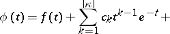
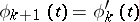
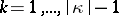
When <img align="absmiddle" border="0" src="https://www.encyclopediaofmath.org/legacyimages/i/i051/i051410/i05141040.png" />, the homogeneous equation corresponding to (4) has exactly <img align="absmiddle" border="0" src="https://www.encyclopediaofmath.org/legacyimages/i/i051/i051410/i05141041.png" /> linearly independent solutions <img align="absmiddle" border="0" src="https://www.encyclopediaofmath.org/legacyimages/i/i051/i051410/i05141042.png" />, which are absolutely-continuous functions on any bounded interval; these solutions can be chosen so that <img align="absmiddle" border="0" src="https://www.encyclopediaofmath.org/legacyimages/i/i051/i051410/i05141043.png" />, <img align="absmiddle" border="0" src="https://www.encyclopediaofmath.org/legacyimages/i/i051/i051410/i05141044.png" /> for <img align="absmiddle" border="0" src="https://www.encyclopediaofmath.org/legacyimages/i/i051/i051410/i05141045.png" />, and <img align="absmiddle" border="0" src="https://www.encyclopediaofmath.org/legacyimages/i/i051/i051410/i05141046.png" />.
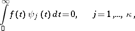
If <img align="absmiddle" border="0" src="https://www.encyclopediaofmath.org/legacyimages/i/i051/i051410/i05141047.png" />, the equation is solvable only if the following condition holds:
| <img align="absmiddle" border="0" src="https://www.encyclopediaofmath.org/legacyimages/i/i051/i051410/i05141048.png" /> | (12) |
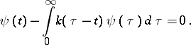
where <img align="absmiddle" border="0" src="https://www.encyclopediaofmath.org/legacyimages/i/i051/i051410/i05141049.png" /> is a system of linearly independent solutions of the transposed homogeneous equation of (4):
| <img align="absmiddle" border="0" src="https://www.encyclopediaofmath.org/legacyimages/i/i051/i051410/i05141050.png" /> | (13) |
Under these conditions, the (unique) solution is given by the formula
| <img align="absmiddle" border="0" src="https://www.encyclopediaofmath.org/legacyimages/i/i051/i051410/i05141051.png" /> |
where
| <img align="absmiddle" border="0" src="https://www.encyclopediaofmath.org/legacyimages/i/i051/i051410/i05141052.png" /> |
| <img align="absmiddle" border="0" src="https://www.encyclopediaofmath.org/legacyimages/i/i051/i051410/i05141053.png" /> |
while the Fourier transforms <img align="absmiddle" border="0" src="https://www.encyclopediaofmath.org/legacyimages/i/i051/i051410/i05141054.png" /> and <img align="absmiddle" border="0" src="https://www.encyclopediaofmath.org/legacyimages/i/i051/i051410/i05141055.png" /> of the functions <img align="absmiddle" border="0" src="https://www.encyclopediaofmath.org/legacyimages/i/i051/i051410/i05141056.png" /> are defined by the equation
| <img align="absmiddle" border="0" src="https://www.encyclopediaofmath.org/legacyimages/i/i051/i051410/i05141057.png" /> |
and the equations (11). Noether's theorem holds for equation (4) (see Singular integral equation).
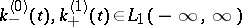
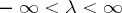
The first significant results in the theory of equations (4) were obtained in [11], where an effective method (the so-called Wiener–Hopf method) for solving the homogeneous equation corresponding to (4) was given under the hypothesis that the kernel and the required solution satisfy the conditions: For some <img align="absmiddle" border="0" src="https://www.encyclopediaofmath.org/legacyimages/i/i051/i051410/i05141058.png" /> both
| <img align="absmiddle" border="0" src="https://www.encyclopediaofmath.org/legacyimages/i/i051/i051410/i05141059.png" /> |
The main point of the Wiener–Hopf method is the idea of factorization of a function <img align="absmiddle" border="0" src="https://www.encyclopediaofmath.org/legacyimages/i/i051/i051410/i05141060.png" /> which is holomorphic in the strip <img align="absmiddle" border="0" src="https://www.encyclopediaofmath.org/legacyimages/i/i051/i051410/i05141061.png" />, that is, the possibility to represent it as a product <img align="absmiddle" border="0" src="https://www.encyclopediaofmath.org/legacyimages/i/i051/i051410/i05141062.png" />, where <img align="absmiddle" border="0" src="https://www.encyclopediaofmath.org/legacyimages/i/i051/i051410/i05141063.png" /> are functions holomorphic in the half-planes <img align="absmiddle" border="0" src="https://www.encyclopediaofmath.org/legacyimages/i/i051/i051410/i05141064.png" /> and <img align="absmiddle" border="0" src="https://www.encyclopediaofmath.org/legacyimages/i/i051/i051410/i05141065.png" />, respectively, and satisfy certain additional requirements. These results have been developed and amplified (see [4]).
A method has been developed for reducing equation (4) to a boundary value problem of linear identification. In this way, equation (4) has been solved under the following hypotheses: <img align="absmiddle" border="0" src="https://www.encyclopediaofmath.org/legacyimages/i/i051/i051410/i05141066.png" />, <img align="absmiddle" border="0" src="https://www.encyclopediaofmath.org/legacyimages/i/i051/i051410/i05141067.png" />, <img align="absmiddle" border="0" src="https://www.encyclopediaofmath.org/legacyimages/i/i051/i051410/i05141068.png" />, <img align="absmiddle" border="0" src="https://www.encyclopediaofmath.org/legacyimages/i/i051/i051410/i05141069.png" />, <img align="absmiddle" border="0" src="https://www.encyclopediaofmath.org/legacyimages/i/i051/i051410/i05141070.png" />, as <img align="absmiddle" border="0" src="https://www.encyclopediaofmath.org/legacyimages/i/i051/i051410/i05141071.png" />, and <img align="absmiddle" border="0" src="https://www.encyclopediaofmath.org/legacyimages/i/i051/i051410/i05141072.png" />, <img align="absmiddle" border="0" src="https://www.encyclopediaofmath.org/legacyimages/i/i051/i051410/i05141073.png" />.
In addition to this, the role of the number <img align="absmiddle" border="0" src="https://www.encyclopediaofmath.org/legacyimages/i/i051/i051410/i05141074.png" /> in solving (4) has been clarified. In earlier articles an analogous role was played by the number of zeros of the analytic function <img align="absmiddle" border="0" src="https://www.encyclopediaofmath.org/legacyimages/i/i051/i051410/i05141075.png" /> in a strip (see ).
Condition (5) is both necessary and sufficient in order that Noether's theorem holds for equation (4). The solution of equation (4) given above simplifies in a number of particular cases important in practice. The asymptotics of the solution have been obtained for special right-hand sides (see [4]).
Equation (4) has also been studied in the case when <img align="absmiddle" border="0" src="https://www.encyclopediaofmath.org/legacyimages/i/i051/i051410/i05141076.png" /> and the Fourier transform <img align="absmiddle" border="0" src="https://www.encyclopediaofmath.org/legacyimages/i/i051/i051410/i05141077.png" /> of the kernel <img align="absmiddle" border="0" src="https://www.encyclopediaofmath.org/legacyimages/i/i051/i051410/i05141078.png" /> has discontinuities of the first kind (see [5]) or is an almost-periodic function (see [2]). In these cases, condition (5) turns out to be insufficient for Noether's theorem to hold.
The validity of the majority of results listed above has also been established for systems of equations of type (4); however, in contrast to the case of a single equation, a system of integral equations of convolution type in the general case cannot be solved explicitly by quadratures (see [6]).
Also related to integral equations of convolution type are paired equations (or dual equations)
| <img align="absmiddle" border="0" src="https://www.encyclopediaofmath.org/legacyimages/i/i051/i051410/i05141079.png" /> | (15) |
| <img align="absmiddle" border="0" src="https://www.encyclopediaofmath.org/legacyimages/i/i051/i051410/i05141080.png" /> |
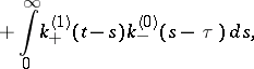
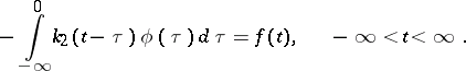
and their transposed equations, so-called integral equations of convolution type with two kernels:
| <img align="absmiddle" border="0" src="https://www.encyclopediaofmath.org/legacyimages/i/i051/i051410/i05141081.png" /> | (16) |
| <img align="absmiddle" border="0" src="https://www.encyclopediaofmath.org/legacyimages/i/i051/i051410/i05141082.png" /> |
Equations (15) have been explicitly solved by quadratures in , and equation (16) in [10].
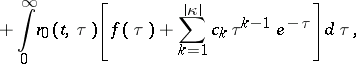
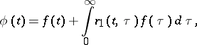
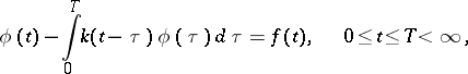
An integral equation of convolution type on a bounded interval,
| <img align="absmiddle" border="0" src="https://www.encyclopediaofmath.org/legacyimages/i/i051/i051410/i05141083.png" /> | (17) |
where <img align="absmiddle" border="0" src="https://www.encyclopediaofmath.org/legacyimages/i/i051/i051410/i05141084.png" />, is called a Fredholm equation (see [7], [9]).
Integral equations of convolution type whose symbol vanishes at a finite number of points and the orders of whose zeros are integers, lend themselves to an explicit solution by quadratures (see [8], [12]).
References
| [1] | B. Noble, "Methods based on the Wiener–Hopf technique for the solution of partial differential equations" , Pergamon (1958) |
| [2] | I.C. [I.Ts. Gokhberg] Gohberg, I.A. Feld'man, "Convolution equations and projection methods for their solution" , Transl. Math. Monogr. , 41 , Amer. Math. Soc. (1974) (Translated from Russian) |
| [3a] | I.M. Rapoport, "On a class of singular integral equations" Dokl. Akad. Nauk. SSSR , 59 : 8 (1948) pp. 1403–1406 (In Russian) |
| [3b] | I.M. Rapoport, Trudy Mat. Inst. Steklov. , 12 (1949) pp. 102–117 |
| [4] | M.G. Krein, "Integral equations on the half-line with kernel depending on the difference of the arguments" Uspekhi Mat. Nauk , 13 : 5 (1958) pp. 3–120 (In Russian) |
| [5] | R.V. Duduchava, "Wiener–Hopf integral operators" Math. Nachr. , 65 : 1 (1975) pp. 59–82 (In Russian) |
| [6] | I.Ts. Gokhberg, M.G. Krein, "Fundamental aspects of deficiency numbers, root numbers and indexes of linear operators" Uspekhi Mat. Nauk , 12 : 2 (1957) pp. 44–118 (In Russian) |
| [7] | M.P. Ganin, "On a Fredholm integral equation whose kernel depends on the difference of two arguments" Izv. Vuzov. Mat. : 2 (1963) pp. 31–43 (In Russian) |
| [8] | F.D. Gakhov, V.I. Smagina, "Exceptional cases of integral equations of convolution type and equations of the first kind" Izv. Akad. Nauk SSSR Ser. Mat. , 26 : 3 (1962) pp. 361–390 (In Russian) |
| [9] | I.B. Simonenko, "On some integro-differential equations of convolution type" Izv. Vuzov. Mat. : 2 (1959) pp. 213–226 (In Russian) |
| [10] | Yu.I. Cherskii, "On some special integral equations" Uchen. Zap. Kazansk. Univ. , 113 : 10 (1953) pp. 43–56 (In Russian) |
| [11] | N. Wiener, E. Hopf, "Ueber eine Klasse singulärer Integralgleichungen" Sitz. Ber. Akad. Wiss. Berlin 30/32 (1931) pp. 696–706 |
| [12] | S. Prössdorf, "Einige Klassen singulärer Gleichungen" , Birkhäuser (1974) |
Comments
See also Abel integral equation, for an example.
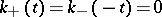
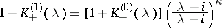
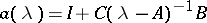
In general, systems of equations of type (4) cannot be solved explicitly. An exception occurs when the symbol <img align="absmiddle" border="0" src="https://www.encyclopediaofmath.org/legacyimages/i/i051/i051410/i05141085.png" /> is a rational matrix function. In that case <img align="absmiddle" border="0" src="https://www.encyclopediaofmath.org/legacyimages/i/i051/i051410/i05141086.png" /> can be written in the form <img align="absmiddle" border="0" src="https://www.encyclopediaofmath.org/legacyimages/i/i051/i051410/i05141087.png" />, where <img align="absmiddle" border="0" src="https://www.encyclopediaofmath.org/legacyimages/i/i051/i051410/i05141088.png" /> is an identity matrix, <img align="absmiddle" border="0" src="https://www.encyclopediaofmath.org/legacyimages/i/i051/i051410/i05141089.png" /> is a square matrix of order <img align="absmiddle" border="0" src="https://www.encyclopediaofmath.org/legacyimages/i/i051/i051410/i05141090.png" />, say, without real eigen values, and <img align="absmiddle" border="0" src="https://www.encyclopediaofmath.org/legacyimages/i/i051/i051410/i05141091.png" /> and <img align="absmiddle" border="0" src="https://www.encyclopediaofmath.org/legacyimages/i/i051/i051410/i05141092.png" /> are (possibly non-square) matrices of appropriate sizes. Such a representation, which comes from mathematical systems theory, is called a realization of <img align="absmiddle" border="0" src="https://www.encyclopediaofmath.org/legacyimages/i/i051/i051410/i05141093.png" />. The system of Wiener–Hopf equations can now be analyzed in terms of <img align="absmiddle" border="0" src="https://www.encyclopediaofmath.org/legacyimages/i/i051/i051410/i05141094.png" />, <img align="absmiddle" border="0" src="https://www.encyclopediaofmath.org/legacyimages/i/i051/i051410/i05141095.png" /> and <img align="absmiddle" border="0" src="https://www.encyclopediaofmath.org/legacyimages/i/i051/i051410/i05141096.png" />. The analysis yields explicit formulas for solutions, as well as explicit formulas for Wiener–Hopf factorization. Interpreting (4) as a system of equations involving a matrix kernel <img align="absmiddle" border="0" src="https://www.encyclopediaofmath.org/legacyimages/i/i051/i051410/i05141097.png" /> and <img align="absmiddle" border="0" src="https://www.encyclopediaofmath.org/legacyimages/i/i051/i051410/i05141098.png" />-vector functions <img align="absmiddle" border="0" src="https://www.encyclopediaofmath.org/legacyimages/i/i051/i051410/i05141099.png" /> and <img align="absmiddle" border="0" src="https://www.encyclopediaofmath.org/legacyimages/i/i051/i051410/i051410100.png" />, one of the major results obtained through this approach reads as follows. For each <img align="absmiddle" border="0" src="https://www.encyclopediaofmath.org/legacyimages/i/i051/i051410/i051410101.png" /> in <img align="absmiddle" border="0" src="https://www.encyclopediaofmath.org/legacyimages/i/i051/i051410/i051410102.png" />, equation (4) has a unique solution <img align="absmiddle" border="0" src="https://www.encyclopediaofmath.org/legacyimages/i/i051/i051410/i051410103.png" /> in <img align="absmiddle" border="0" src="https://www.encyclopediaofmath.org/legacyimages/i/i051/i051410/i051410104.png" /> if and only if <img align="absmiddle" border="0" src="https://www.encyclopediaofmath.org/legacyimages/i/i051/i051410/i051410105.png" /> has no real eigen values and <img align="absmiddle" border="0" src="https://www.encyclopediaofmath.org/legacyimages/i/i051/i051410/i051410106.png" /> is the direct sum of <img align="absmiddle" border="0" src="https://www.encyclopediaofmath.org/legacyimages/i/i051/i051410/i051410107.png" /> and <img align="absmiddle" border="0" src="https://www.encyclopediaofmath.org/legacyimages/i/i051/i051410/i051410108.png" />, where <img align="absmiddle" border="0" src="https://www.encyclopediaofmath.org/legacyimages/i/i051/i051410/i051410109.png" /> and <img align="absmiddle" border="0" src="https://www.encyclopediaofmath.org/legacyimages/i/i051/i051410/i051410110.png" /> are the spectral subspaces corresponding to the eigen values of <img align="absmiddle" border="0" src="https://www.encyclopediaofmath.org/legacyimages/i/i051/i051410/i051410111.png" /> and <img align="absmiddle" border="0" src="https://www.encyclopediaofmath.org/legacyimages/i/i051/i051410/i051410112.png" /> located in the upper and lower half-planes, respectively. Furthermore, in that case the symbol <img align="absmiddle" border="0" src="https://www.encyclopediaofmath.org/legacyimages/i/i051/i051410/i051410113.png" /> admits a (canonical Wiener–Hopf) factorization <img align="absmiddle" border="0" src="https://www.encyclopediaofmath.org/legacyimages/i/i051/i051410/i051410114.png" /> with
| <img align="absmiddle" border="0" src="https://www.encyclopediaofmath.org/legacyimages/i/i051/i051410/i051410115.png" /> |
| <img align="absmiddle" border="0" src="https://www.encyclopediaofmath.org/legacyimages/i/i051/i051410/i051410116.png" /> |
| <img align="absmiddle" border="0" src="https://www.encyclopediaofmath.org/legacyimages/i/i051/i051410/i051410117.png" /> |
| <img align="absmiddle" border="0" src="https://www.encyclopediaofmath.org/legacyimages/i/i051/i051410/i051410118.png" /> |
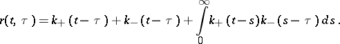
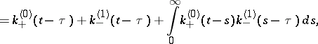
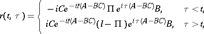
and the resolvent kernel <img align="absmiddle" border="0" src="https://www.encyclopediaofmath.org/legacyimages/i/i051/i051410/i051410119.png" /> of (4) is given by
| <img align="absmiddle" border="0" src="https://www.encyclopediaofmath.org/legacyimages/i/i051/i051410/i051410120.png" /> |
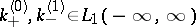
where <img align="absmiddle" border="0" src="https://www.encyclopediaofmath.org/legacyimages/i/i051/i051410/i051410121.png" /> is the projection of <img align="absmiddle" border="0" src="https://www.encyclopediaofmath.org/legacyimages/i/i051/i051410/i051410122.png" /> along <img align="absmiddle" border="0" src="https://www.encyclopediaofmath.org/legacyimages/i/i051/i051410/i051410123.png" /> onto <img align="absmiddle" border="0" src="https://www.encyclopediaofmath.org/legacyimages/i/i051/i051410/i051410124.png" />. Of particular interest is the situation where the symbol is self-adjoint (cf. [a11]). For further details and additional results (also on non-canonical Wiener–Hopf factorization) see [a1], [a2], [a7], and [a9]. Generalizations are possible to certain classes of non-rational symbols. For these classes, the realizations involve infinite-dimensional, possibly unbounded, operators (cf. [a3], [a4] and [a9]). For applications to the transport equation and abstract kinetic theory, see [a2], [a8] and [a10]; for applications to <img align="absmiddle" border="0" src="https://www.encyclopediaofmath.org/legacyimages/i/i051/i051410/i051410125.png" /> control theory, cf. [a6].
See also Fredholm operator.
References
| [a1] | H. Bart, "Transfer functions and operator theory" Linear Alg. Appl. , 84 (1986) pp. 33–61 |
| [a2] | H. Bart, I. Gohberg, M.A. Kaashoek, "Minimal factorization of matrix and operation functions" , Birkhäuser (1979) |
| [a3] | H Bart, I. Gohberg, M.A. Kaashoek, "Fredholm theory of Wiener–Hopf equations in terms of realization of their symbols" Integr. Eq. Oper. Theory , 8 (1985) pp. 590–613 |
| [a4] | H Bart, I. Gohberg, M.A. Kaashoek, "Wiener–Hopf factorization, inverse Fourier transforms and exponentially dichotomous operators" J. Funct. Anal. , 68 (1986) pp. 1–42 |
| [a5] | K. Clancey, I. Gohberg, "Factorization of matrix functions and singular integral operators" , Birkhäuser (1981) |
| [a6] | B.A. Francis, "A course in <img align="absmiddle" border="0" src="https://www.encyclopediaofmath.org/legacyimages/i/i051/i051410/i051410126.png" /> control theory" , Lect. notes in control and inform. science , 88 , Springer (1987) |
| [a7] | I. Gohberg (ed.) M.A. Kaashoek (ed.) , Constructive methods of Wiener–Hopf factorization , Birkhäuser (1986) |
| [a8] | W. Greenberg, C. van der Mee, V. Protopopescu, "Boundary value problems in abstract kinetic theory" , Birkhäuser (1987) |
| [a9] | M.A. Kaashoek, "Minimal factorization, linear systems and integral operators" S.S. Power (ed.) , Operators and function theory , Reidel (1985) pp. 41–86 |
| [a10] | H.G. Kaper, C.G. Lekkerkerker, J. Hejtmanek, "Spectral methods in linear transport theory" , Birkhäuser (1982) |
| [a11] | A.C.M. Ran, "Minimal factorization of selfadjoint rational matrix functions" Integr. Eq. Oper. Theory , 5 (1982) pp. 850–869 |
| [a12] | A.G. Ramm, "Theory and applications of some new classes of integral equations" , Springer (1980) |
| [a13] | A. Ziolkowski, "Deconvolution" , Reidel (1984) |
 |  |
