Jacket matrix

From HandWiki

In mathematics, a jacket matrix is a square symmetric matrix [math]\displaystyle{ A= (a_{ij}) }[/math] of order n if its entries are non-zero and real, complex, or from a finite field, and
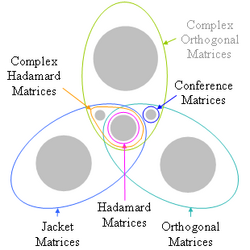
Hierarchy of matrix types
[math]\displaystyle{ \ AB=BA=I_n }[/math]

where In is the identity matrix, and

[math]\displaystyle{ \ B ={1 \over n}(a_{ij}^{-1})^T. }[/math]

where T denotes the transpose of the matrix.

In other words, the inverse of a jacket matrix is determined its element-wise or block-wise inverse. The definition above may also be expressed as:

[math]\displaystyle{ \forall u,v \in \{1,2,\dots,n\}:~a_{iu},a_{iv} \neq 0, ~~~~ \sum_{i=1}^n a_{iu}^{-1}\,a_{iv} = \begin{cases} n, & u = v\\ 0, & u \neq v \end{cases} }[/math]

The jacket matrix is a generalization of the Hadamard matrix; it is a diagonal block-wise inverse matrix.

Motivation

n .... −2, −1, 0 1, 2,..... logarithm
2n ....[math]\displaystyle{ \ {1 \over 4}, {1 \over 2}, }[/math] 1, 2, 4, ... series

As shown in the table, i.e. in the series, for example with n=2, forward: [math]\displaystyle{ 2^2 = 4 }[/math], inverse : [math]\displaystyle{ (2^2)^{-1}={1 \over 4} }[/math], then, [math]\displaystyle{ 4*{1\over 4}=1 }[/math]. That is, there exists an element-wise inverse.

Example 1.

[math]\displaystyle{ A = \left[ \begin{array}{rrrr} 1 & 1 & 1 & 1 \\ 1 & -2 & 2 & -1 \\ 1 & 2 & -2 & -1 \\ 1 & -1 & -1 & 1 \\ \end{array} \right], }[/math]:[math]\displaystyle{ B ={1 \over 4} \left[ \begin{array}{rrrr} 1 & 1 & 1 & 1 \\[6pt] 1 & -{1 \over 2} & {1 \over 2} & -1 \\[6pt] 1 & {1 \over 2} & -{1 \over 2} & -1 \\[6pt] 1 & -1 & -1 & 1\\[6pt] \end{array} \right]. }[/math]

or more general

[math]\displaystyle{ A = \left[ \begin{array}{rrrr} a & b & b & a \\ b & -c & c & -b \\ b & c & -c & -b \\ a & -b & -b & a \end{array} \right], }[/math]:[math]\displaystyle{ B = {1 \over 4} \left[ \begin{array}{rrrr} {1 \over a} & {1 \over b} & {1 \over b} & {1 \over a} \\[6pt] {1 \over b} & -{1 \over c} & {1 \over c} & -{1 \over b} \\[6pt] {1 \over b} & {1 \over c} & -{1 \over c} & -{1 \over b} \\[6pt] {1 \over a} & -{1 \over b} & -{1 \over b} & {1 \over a} \end{array} \right], }[/math]

Example 2.

For m x m matrices, [math]\displaystyle{ \mathbf {A_j}, }[/math]

[math]\displaystyle{ \mathbf {A_j}=\mathrm{diag}(A_1, A_2,.. A_n ) }[/math] denotes an mn x mn block diagonal Jacket matrix.

[math]\displaystyle{ J_4 = \left[ \begin{array}{rrrr} I_2 & 0 & 0 & 0 \\ 0 & \cos\theta & -\sin\theta & 0 \\ 0 & \sin\theta & \cos\theta & 0 \\ 0 & 0 & 0 & I_2 \end{array} \right], }[/math] [math]\displaystyle{ \ J^T_4 J_4 =J_4 J^T_4=I_4. }[/math]

Example 3.

Euler's formula:

[math]\displaystyle{ e^{i \pi} + 1 = 0 }[/math], [math]\displaystyle{ e^{i \pi} =\cos{ \pi} +i\sin{\pi}=-1 }[/math] and [math]\displaystyle{ e^{-i \pi} =\cos{ \pi} - i\sin{\pi}=-1 }[/math].

Therefore,

[math]\displaystyle{ e^{i \pi}e^{-i \pi}=(-1)(\frac{1}{-1})=1 }[/math].

Also,

[math]\displaystyle{ y=e^{x} }[/math]
[math]\displaystyle{ \frac{dy}{dx}=e^{x} }[/math],[math]\displaystyle{ \frac{dy}{dx}\frac{dx}{dy}=e^{x}\frac{1}{e^{x}}=1 }[/math].

Finally,

A·B = B·A = I

Example 4.

Consider  [math]\displaystyle{ [\mathbf {A}]_N }[/math] be 2x2 block matrices of order [math]\displaystyle{ N=2p }[/math] 
[math]\displaystyle{ [\mathbf {A}]_N= \left[ \begin{array}{rrrr} \mathbf {A}_0 & \mathbf {A}_1 \\ \mathbf {A}_1 & \mathbf {A}_0 \\ \end{array} \right], }[/math].

If [math]\displaystyle{ [\mathbf {A}_0]_p }[/math] and [math]\displaystyle{ [\mathbf {A}_1]_p }[/math] are pxp Jacket matrix, then [math]\displaystyle{ [A]_N }[/math] is a block circulant matrix if and only if [math]\displaystyle{ \mathbf {A}_0 \mathbf {A}_1^{rt}+\mathbf {A}_1^{rt}\mathbf {A}_0 }[/math], where rt denotes the reciprocal transpose.

Example 5.

Let [math]\displaystyle{ \mathbf {A}_0= \left[ \begin{array}{rrrr} -1 & 1 \\ 1 & 1\\ \end{array} \right], }[/math] and [math]\displaystyle{ \mathbf {A}_1= \left[ \begin{array}{rrrr} -1 & -1 \\ -1 & 1\\ \end{array} \right], }[/math], then the matrix [math]\displaystyle{ [\mathbf {A}]_N }[/math] is given by

[math]\displaystyle{ [\mathbf {A}]_4= \left[ \begin{array}{rrrr} \mathbf {A}_0 & \mathbf {A}_1 \\ \mathbf {A}_0 & \mathbf {A}_1 \\ \end{array} \right] =\left[ \begin{array}{rrrr} -1 & 1 & -1 & -1\\ 1 & 1 & -1 & 1 \\ -1 & 1 & -1 & -1 \\ 1 & 1 & -1 & 1 \\ \end{array} \right], }[/math],
[math]\displaystyle{ [\mathbf {A}]_4 }[/math][math]\displaystyle{ \left[ \begin{array}{rrrr} U & C & A & G\\ \end{array} \right]^T\otimes\left[ \begin{array}{rrrr} U & C & A & G\\ \end{array} \right]\otimes\left[ \begin{array}{rrrr} U & C & A & G\\ \end{array} \right]^T, }[/math]

where U, C, A, G denotes the amount of the DNA nucleobases and the matrix [math]\displaystyle{ [\mathbf {A}]_4 }[/math] is the block circulant Jacket matrix which leads to the principle of the Antagonism with Nirenberg Genetic Code matrix.

References

[1] Moon Ho Lee, "The Center Weighted Hadamard Transform", IEEE Transactions on Circuits Syst. Vol. 36, No. 9, PP. 1247–1249, Sept. 1989.

[2] Kathy Horadam, Hadamard Matrices and Their Applications, Princeton University Press, UK, Chapter 4.5.1: The jacket matrix construction, PP. 85–91, 2007.

[3] Moon Ho Lee, Jacket Matrices: Constructions and Its Applications for Fast Cooperative Wireless Signal Processing, LAP LAMBERT Publishing, Germany, Nov. 2012.

[4] Moon Ho Lee, et. al., "MIMO Communication Method and System using the Block Circulant Jacket Matrix," US patent, no. US 009356671B1, May, 2016.

[5] S. K. Lee and M. H. Lee, “The COVID-19 DNA-RNA Genetic Code Analysis Using Information Theory of Double Stochastic Matrix,” IntechOpen, Book Chapter, April 17, 2022. [Available in Online: https://www.intechopen.com/chapters/81329].

External links