Linear inequality

Short description: Inequality which involves a linear function

In mathematics a linear inequality is an inequality which involves a linear function. A linear inequality contains one of the symbols of inequality:

• < less than
• > greater than
• ≤ less than or equal to
• ≥ greater than or equal to
• ≠ not equal to

A linear inequality looks exactly like a linear equation, with the inequality sign replacing the equality sign.

Linear inequalities of real numbers

Two-dimensional linear inequalities

Graph of linear inequality:
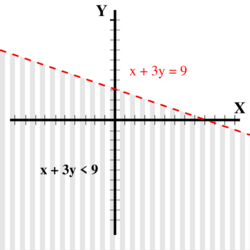
x + 3y < 9

Two-dimensional linear inequalities are expressions in two variables of the form:

[math]\displaystyle{ ax + by \lt c \text{ and } ax + by \geq c, }[/math]

where the inequalities may either be strict or not. The solution set of such an inequality can be graphically represented by a half-plane (all the points on one "side" of a fixed line) in the Euclidean plane. The line that determines the half-planes (ax + by = c) is not included in the solution set when the inequality is strict. A simple procedure to determine which half-plane is in the solution set is to calculate the value of ax + by at a point (x₀, y₀) which is not on the line and observe whether or not the inequality is satisfied.

For example, to draw the solution set of x + 3y < 9, one first draws the line with equation x + 3y = 9 as a dotted line, to indicate that the line is not included in the solution set since the inequality is strict. Then, pick a convenient point not on the line, such as (0,0). Since 0 + 3(0) = 0 < 9, this point is in the solution set, so the half-plane containing this point (the half-plane "below" the line) is the solution set of this linear inequality.

Linear inequalities in general dimensions

In Rⁿ linear inequalities are the expressions that may be written in the form

[math]\displaystyle{ f(\bar{x}) \lt b }[/math] or [math]\displaystyle{ f(\bar{x}) \leq b, }[/math]

where f is a linear form (also called a linear functional), [math]\displaystyle{ \bar{x} = (x_1,x_2,\ldots,x_n) }[/math] and b a constant real number.

More concretely, this may be written out as

[math]\displaystyle{ a_1 x_1 + a_2 x_2 + \cdots + a_n x_n \lt b }[/math]

or

[math]\displaystyle{ a_1 x_1 + a_2 x_2 + \cdots + a_n x_n \leq b. }[/math]

Here [math]\displaystyle{ x_1, x_2,...,x_n }[/math] are called the unknowns, and [math]\displaystyle{ a_{1}, a_{2},..., a_{n} }[/math] are called the coefficients.

Alternatively, these may be written as

[math]\displaystyle{ g(x) \lt 0 \, }[/math] or [math]\displaystyle{ g(x) \leq 0, }[/math]

where g is an affine function.

That is

[math]\displaystyle{ a_0 + a_1 x_1 + a_2 x_2 + \cdots + a_n x_n \lt 0 }[/math]

or

[math]\displaystyle{ a_0 + a_1 x_1 + a_2 x_2 + \cdots + a_n x_n \leq 0. }[/math]

Note that any inequality containing a "greater than" or a "greater than or equal" sign can be rewritten with a "less than" or "less than or equal" sign, so there is no need to define linear inequalities using those signs.

Systems of linear inequalities

A system of linear inequalities is a set of linear inequalities in the same variables:

[math]\displaystyle{ \begin{alignat}{7} a_{11} x_1 &&\; + \;&& a_{12} x_2 &&\; + \cdots + \;&& a_{1n} x_n &&\; \leq \;&&& b_1 \\ a_{21} x_1 &&\; + \;&& a_{22} x_2 &&\; + \cdots + \;&& a_{2n} x_n &&\; \leq \;&&& b_2 \\ \vdots\;\;\; && && \vdots\;\;\; && && \vdots\;\;\; && &&& \;\vdots \\ a_{m1} x_1 &&\; + \;&& a_{m2} x_2 &&\; + \cdots + \;&& a_{mn} x_n &&\; \leq \;&&& b_m \\ \end{alignat} }[/math]

Here [math]\displaystyle{ x_1,\ x_2,...,x_n }[/math] are the unknowns, [math]\displaystyle{ a_{11},\ a_{12},...,\ a_{mn} }[/math] are the coefficients of the system, and [math]\displaystyle{ b_1,\ b_2,...,b_m }[/math] are the constant terms.

This can be concisely written as the matrix inequality

[math]\displaystyle{ Ax \leq b, }[/math]

where A is an m×n matrix, x is an n×1 column vector of variables, and b is an m×1 column vector of constants.

In the above systems both strict and non-strict inequalities may be used.

• Not all systems of linear inequalities have solutions.

Variables can be eliminated from systems of linear inequalities using Fourier–Motzkin elimination.

Applications

Polyhedra

The set of solutions of a real linear inequality constitutes a half-space of the 'n'-dimensional real space, one of the two defined by the corresponding linear equation.

The set of solutions of a system of linear inequalities corresponds to the intersection of the half-spaces defined by individual inequalities. It is a convex set, since the half-spaces are convex sets, and the intersection of a set of convex sets is also convex. In the non-degenerate cases this convex set is a convex polyhedron (possibly unbounded, e.g., a half-space, a slab between two parallel half-spaces or a polyhedral cone). It may also be empty or a convex polyhedron of lower dimension confined to an affine subspace of the n-dimensional space Rⁿ.

Linear programming

A linear programming problem seeks to optimize (find a maximum or minimum value) a function (called the objective function) subject to a number of constraints on the variables which, in general, are linear inequalities. The list of constraints is a system of linear inequalities.

Generalization

The above definition requires well-defined operations of addition, multiplication and comparison; therefore, the notion of a linear inequality may be extended to ordered rings, and in particular to ordered fields.

Sources

• Angel, Allen R.; Porter, Stuart R. (1989), A Survey of Mathematics with Applications (3rd ed.), Addison-Wesley, ISBN 0-201-13696-1 
• Miller, Charles D.; Heeren, Vern E. (1986), Mathematical Ideas (5th ed.), Scott, Foresman, ISBN 0-673-18276-2, https://archive.org/details/mathematicalidea0000mill 

External links

• Khan Academy: Linear inequalities, free online micro lectures

References

- ↑ Miller & Heeren 1986, p. 355
- ↑ Technically, for this statement to be correct both a and b can not simultaneously be zero. In that situation, the solution set is either empty or the entire plane.
- ↑ Angel & Porter 1989, p. 310
- ↑ In the 2-dimensional case, both linear forms and affine functions are historically called linear functions because their graphs are lines. In other dimensions, neither type of function has a graph which is a line, so the generalization of linear function in two dimensions to higher dimensions is done by means of algebraic properties and this causes the split into two types of functions. However, the difference between affine functions and linear forms is just the addition of a constant.
- ↑ Gärtner, Bernd; Matoušek, Jiří (2006). Understanding and Using Linear Programming. Berlin: Springer. ISBN 3-540-30697-8.
- ↑ Angel & Porter 1989, p. 373