Modern Hopfield Network

Short description: Neural networks

Hopfield Networks are recurrent neural networks with dynamical trajectories converging to fixed point attractor states and described by an energy function. The state of each model neuron [math]\displaystyle{ i }[/math] is defined by a time-dependent variable [math]\displaystyle{ V_i }[/math], which can be chosen to be either discrete or continuous. A complete model describes the mathematics of how the future state of activity of each neuron depends on the known present or previous activity of all the neurons.

In the original Hopfield model of associative memory, the variables were binary, and the dynamics were described by a one-at-a-time update of the state of the neurons. An energy function quadratic in the [math]\displaystyle{ V_i }[/math] was defined, and the dynamics consisted of changing the activity of each single neuron [math]\displaystyle{ i }[/math] only if doing so would lower the total energy of the system. This same idea was extended to the case of [math]\displaystyle{ V_i }[/math] being a continuous variable representing the output of neuron [math]\displaystyle{ i }[/math], and [math]\displaystyle{ V_i }[/math] being a monotonic function of an input current. The dynamics became expressed as a set of first-order differential equations for which the "energy" of the system always decreased. The energy in the continuous case has one term which is quadratic in the [math]\displaystyle{ V_i }[/math] (as in the binary model), and a second term which depends on the gain function (neuron's activation function). While having many desirable properties of associative memory, both of these classical systems suffer from a small memory storage capacity, which scales linearly with the number of input features.

Dense Associative Memories (also known as the Modern Hopfield Networks) are generalizations of the classical Hopfield Networks that break the linear scaling relationship between the number of input features and the number of stored memories. This is achieved by introducing stronger non-linearities (either in the energy function or neurons’ activation functions) leading to super-linear (even an exponential) memory storage capacity as a function of the number of feature neurons. The network still requires a sufficient number of hidden neurons.

The key theoretical idea behind the Modern Hopfield Networks is to use an energy function and an update rule that is more sharply peaked around the stored memories in the space of neuron’s configurations compared to the classical Hopfield Network.

Discrete Variables

A simple example of the Modern Hopfield Network can be written in terms of binary variables [math]\displaystyle{ V_i }[/math] that represent the active [math]\displaystyle{ V_i=+1 }[/math] and inactive [math]\displaystyle{ V_i=-1 }[/math] state of the model neuron [math]\displaystyle{ i }[/math].[math]\displaystyle{ E = - \sum\limits_{\mu = 1}^{N_\text{mem}} F\Big(\sum\limits_{i=1}^{N_f}\xi_{\mu i} V_i\Big) }[/math]In this formula the weights [math]\displaystyle{ \xi_{\mu i} }[/math] represent the matrix of memory vectors (index [math]\displaystyle{ \mu = 1...N_\text{mem} }[/math] enumerates different memories, and index [math]\displaystyle{ i=1...N_f }[/math] enumerates the content of each memory corresponding to the [math]\displaystyle{ i }[/math]-th feature neuron), and the function [math]\displaystyle{ F(x) }[/math] is a rapidly growing non-linear function. The update rule for individual neurons (in the asynchronous case) can be written in the following form [math]\displaystyle{ V^{(t+1)}_i = Sign\bigg[ \sum\limits_{\mu=1}^{N_\text{mem}} \bigg(F\Big(\xi_{\mu i} + \sum\limits_{j\neq i}\xi_{\mu j} V^{(t)}_j\Big) - F\Big(-\xi_{\mu i} + \sum\limits_{j\neq i}\xi_{\mu j} V^{(t)}_j\Big) \bigg)\bigg] }[/math]which states that in order to calculate the updated state of the [math]\displaystyle{ i }[/math]-th neuron the network compares two energies: the energy of the network with the [math]\displaystyle{ i }[/math]-th neuron in the ON state and the energy of the network with the [math]\displaystyle{ i }[/math]-th neuron in the OFF state, given the states of the remaining neuron. The updated state of the [math]\displaystyle{ i }[/math]-th neuron selects the state that has the lowest of the two energies.

In the limiting case when the non-linear energy function is quadratic [math]\displaystyle{ F(x) = x^2 }[/math] these equations reduce to the familiar energy function and the update rule for the classical binary Hopfield Network.

The memory storage capacity of these networks can be calculated for random binary patterns. For the power energy function [math]\displaystyle{ F(x)=x^n }[/math] the maximal number of memories that can be stored and retrieved from this network without errors is given by[math]\displaystyle{ N^{max}_{\text{mem}}\approx \frac{1}{2 (2n-3)!!} \frac{N_f^{n-1}}{\ln(N_f)} }[/math]For an exponential energy function [math]\displaystyle{ F(x)=e^x }[/math] the memory storage capacity is exponential in the number of feature neurons[math]\displaystyle{ N^{max}_{\text{mem}}\approx 2^{N_f/2} }[/math]

Continuous Variables

Fig.1 An example of a continuous Modern Hopfield Network with [math]\displaystyle{ N_f=5 }[/math] feature neurons and [math]\displaystyle{ N_\text{mem}=11 }[/math] memory (hidden) neurons with symmetric synaptic connections between them.

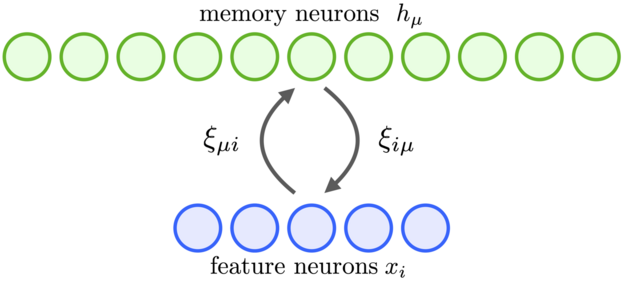
Modern Hopfield Networks or Dense Associative Memories can be best understood in continuous variables and continuous time. Consider the network architecture, shown in Fig.1, and the equations for neuron's states evolution

[math]\displaystyle{ \begin{cases} \tau_f \frac{d x_i}{dt} = \sum\limits_{\mu=1}^{N_h} \xi_{i \mu} f_\mu - x_i + I_i\\ \tau_h \frac{d h_\mu}{dt} = \sum\limits_{i=1}^{N_f} \xi_{\mu i} g_i - h_\mu \end{cases} }[/math]

(1)

where the currents of the feature neurons are denoted by [math]\displaystyle{ x_i }[/math], and the currents of the memory neurons are denoted by [math]\displaystyle{ h_\mu }[/math] ([math]\displaystyle{ h }[/math] stands for hidden neurons). There are no synaptic connections among the feature neurons or the memory neurons. A matrix [math]\displaystyle{ \xi_{\mu i} }[/math] denotes the strength of synapses from a feature neuron [math]\displaystyle{ i }[/math] to the memory neuron [math]\displaystyle{ \mu }[/math]. The synapses are assumed to be symmetric, so that the same value characterizes a different physical synapse from the memory neuron [math]\displaystyle{ \mu }[/math] to the feature neuron [math]\displaystyle{ i }[/math]. The outputs of the memory neurons and the feature neurons are denoted by [math]\displaystyle{ f_\mu }[/math] and [math]\displaystyle{ g_i }[/math], which are non-linear functions of the corresponding currents. In general these outputs can depend on the currents of all the neurons in that layer so that [math]\displaystyle{ f_\mu = f(\{h_\mu\}) }[/math] and [math]\displaystyle{ g_i = g(\{x_i\}) }[/math]. It is convenient to define these activation function as derivatives of the Lagrangian functions for the two groups of neurons

[math]\displaystyle{ f_\mu = \frac{\partial L_h}{\partial h_\mu},\ \ \ \ \text{and}\ \ \ \ g_i = \frac{\partial L_v}{\partial x_i} }[/math]

(2)

This way the specific form of the equations for neuron's states is completely defined once the Lagrangian functions are specified. Finally, the time constants for the two groups of neurons are denoted by [math]\displaystyle{ \tau_f }[/math] and [math]\displaystyle{ \tau_h }[/math], [math]\displaystyle{ I_i }[/math] is the input current to the network that can be driven by the presented data.

Fig.2 Effective theory on the feature neurons for various common choices of the Lagrangian functions. Model A reduces to the models studied in depending on the choice of the activation function, model B reduces to the model studied in, model C reduces to the model of.

General systems of non-linear differential equations can have many complicated behaviors that can depend on the choice of the non-linearities and the initial conditions. For Hopfield Networks, however, this is not the case - the dynamical trajectories always converge to a fixed point attractor state. This property is achieved because these equations are specifically engineered so that they have an underlying energy function

[math]\displaystyle{ E(t) = \Big[\sum\limits_{i=1}^{N_f} (x_i-I_i) g_i - L_x \Big] + \Big[\sum\limits_{\mu=1}^{N_h} h_\mu f_\mu - L_h \Big] - \sum\limits_{\mu, i} f_\mu \xi_{\mu i} g_i }[/math]

(3)

The terms grouped into square brackets represent a Legendre transform of the Lagrangian function with respect to the states of the neurons. If the Hessian matrices of the Lagrangian functions are positive semi-definite, the energy function is guaranteed to decrease on the dynamical trajectory

[math]\displaystyle{ \frac{dE(t)}{dt}= - \tau_f \sum\limits_{i,j=1}^{N_f} \frac{d x_i}{dt} \frac{\partial^2 L_x}{\partial x_i \partial x_j} \frac{d x_j}{dt} - \tau_h \sum\limits_{\mu,\nu = 1}^{N_h} \frac{d h_\mu}{dt} \frac{\partial^2 L_h}{\partial h_\mu \partial h_\nu} \frac{d h_\nu}{dt} \leq 0 }[/math]

(4)

This property makes it possible to prove that the system of dynamical equations describing temporal evolution of neurons' activities will eventually reach a fixed point attractor state.

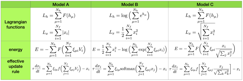
In certain situations one can assume that the dynamics of hidden neurons equilibrates at a much faster time scale compared to the feature neurons, [math]\displaystyle{ \tau_h\ll\tau_f }[/math]. In this case the steady state solution of the second equation in the system (1) can be used to express the currents of the hidden units through the outputs of the feature neurons. This makes it possible to reduce the general theory (1) to an effective theory for feature neurons only. The resulting effective update rules and the energies for various common choices of the Lagrangian functions are shown in Fig.2. In the case of log-sum-exponential Lagrangian function the update rule (if applied once) for the states of the feature neurons is the attention mechanism commonly used in many modern AI systems (see Ref. for the derivation of this result from the continuous time formulation).

Relationship to Classical Hopfield Network with Continuous Variables

Classical formulation of continuous Hopfield Networks can be understood as a special limiting case of the Modern Hopfield Networks with one hidden layer. Continuous Hopfield Networks for neurons with graded response are typically described by the dynamical equations

[math]\displaystyle{ \tau_f \frac{d x_i}{dt} = \sum\limits_{j=1}^{N_f}T_{ij} V_j - x_i + I_i }[/math]

(5)

and the energy function

[math]\displaystyle{ E = -\frac{1}{2}\sum\limits_{i,j=1}^{N_f} T_{ij} V_i V_j - \sum\limits_{i=1}^{N_f} V_i I_i + \sum\limits_{i=1}^{N_f} \int\limits^{V_i} g^{-1}(z)dz }[/math]

(6)

where [math]\displaystyle{ V_i = g(x_i) }[/math], and [math]\displaystyle{ g^{-1}(z) }[/math] is the inverse of the activation function [math]\displaystyle{ g(x) }[/math]. This model is a special limit of the class of models that is called models A, with the following choice of the Lagrangian functions

[math]\displaystyle{ L_v = \sum\limits_{i=1}^{N_f}\int\limits^{x_i} g(x) dx,\ \ \ \ \ \text{and}\ \ \ \ \ L_h = \frac{1}{2} \sum\limits_{\mu=1}^{N_h} h_\mu^2 }[/math]

(7)

that, according to the definition (2), leads to the activation functions

[math]\displaystyle{ V_i = g(x_i), \ \ \ \ \ \text{and}\ \ \ \ \ f_\mu = h_\mu }[/math]

(8)

If we integrate out the hidden neurons the system of equations (1) reduces to the equations on the feature neurons (5) with [math]\displaystyle{ T_{ij} = \sum\limits_{\mu=1}^{N_h} \xi_{\mu i }\xi_{\mu j} }[/math], and the general expression for the energy (3) reduces to the effective energy

[math]\displaystyle{ E = -\frac{1}{2} \sum\limits_{i,j=1}^{N_f} T_{ij} V_i V_j - \sum\limits_{i=1}^{N_f} V_i I_i +\sum\limits_{i=1}^{N_f} \Big( x_i V_i - \int\limits^{x_i} g(x)dx \Big) }[/math]

(9)

While the first two terms in equation (6) are the same as those in equation (9), the third terms look superficially different. In equation (9) it is a Legendre transform of the Lagrangian for the feature neurons, while in (6) the third term is an integral of the inverse activation function. Nevertheless, these two expressions are in fact equivalent, since the derivatives of a function and its Legendre transform are inverse functions of each other. The easiest way to see that these two terms are equal explicitly is to differentiate each one with respect to [math]\displaystyle{ x_i }[/math]. The results of these differentiations for both expressions are equal to [math]\displaystyle{ x_i g(x_i)' }[/math]. Thus, the two expressions are equal up to an additive constant. This completes the proof that the classical Hopfield Network with continuous states is a special limiting case of the Modern Hopfield Network (1) with energy (3).

General Formulation of the Modern Hopfield Network

Fig.3 The connectivity diagram of the fully-connected Modern Hopfield Network consisting of five neurons. The synaptic weights are described by a symmetric matrix [math]\displaystyle{ W_{IJ} }[/math].

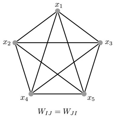
Biological neural networks have a large degree of heterogeneity in terms of different cell types. This section describes a mathematical model of a fully connected Modern Hopfield Network assuming the extreme degree of heterogeneity: every single neuron is different. Specifically, an energy function and the corresponding dynamical equations are described assuming that each neuron has its own activation function and kinetic time scale. The network is assumed to be fully connected, so that every neuron is connected to every other neuron using a symmetric matrix of weights [math]\displaystyle{ W_{IJ} }[/math], indices [math]\displaystyle{ I }[/math] and [math]\displaystyle{ J }[/math] enumerate different neurons in the network, see Fig.3. The easiest way to mathematically formulate this problem is to define the architecture through a Lagrangian function [math]\displaystyle{ L(\{x_I\}) }[/math] that depends on the activities of all the neurons in the network. The activation function for each neuron is defined as a partial derivative of the Lagrangian with respect to that neuron's activity

[math]\displaystyle{ g_I = \frac{\partial L}{\partial x_I} }[/math]

(10)

From the biological perspective one can think about [math]\displaystyle{ g_I }[/math] as an axonal output of the neuron [math]\displaystyle{ I }[/math]. In the simplest case, when the Lagrangian is additive for different neurons, this definition results in the activation that is a non-linear function of that neuron's activity. For non-additive Lagrangians this activation function can depend on the activities of a group of neurons. For instance, it can contain contrastive (softmax) or divisive normalization. The dynamical equations describing temporal evolution of a given neuron are given by

[math]\displaystyle{ \tau_I \frac{dx_I}{dt} = \sum\limits_{J=1}^N W_{IJ} g_J - x_I }[/math]

(11)

This equation belongs to the class of models called firing rate models in neuroscience. Each neuron [math]\displaystyle{ I }[/math] collects the axonal outputs [math]\displaystyle{ g_J }[/math] from all the neurons, weights them with the synaptic coefficients [math]\displaystyle{ W_{IJ} }[/math] and produces its own time-dependent activity [math]\displaystyle{ x_I }[/math]. The temporal evolution has a time constant [math]\displaystyle{ \tau_I }[/math], which in general can be different for every neuron. This network has a global energy function

[math]\displaystyle{ E = \sum\limits_{I=1}^N x_I g_I - L - \frac{1}{2} \sum\limits_{I,J=1}^N g_I W_{IJ} g_J }[/math]

(12)

where the first two terms represent the Legendre transform of the Lagrangian function with respect to the neurons' currents [math]\displaystyle{ x_I }[/math]. The temporal derivative of this energy function can be computed on the dynamical trajectories leading to (see for details)

[math]\displaystyle{ \frac{dE}{dt} = - \sum\limits_{I,K=1}^N \frac{dx_I}{dt} M_{IK} \frac{dx_K}{dt}\leq 0, \ \ \ \ \text{where}\ \ \ \ M_{IK} = \tau_I \frac{\partial^2 L }{\partial x_I \partial x_K} }[/math]

(13)

The last inequality sign holds provided that the matrix [math]\displaystyle{ M_{IK} }[/math] (or its symmetric part) is positive semi-definite. If, in addition to this, the energy function is bounded from below the non-linear dynamical equations are guaranteed to converge to a fixed point attractor state. The advantage of formulating this network in terms of the Lagrangian functions is that it makes it possible to easily experiment with different choices of the activation functions and different architectural arrangements of neurons. For all those flexible choices the conditions of convergence are determined by the properties of the matrix [math]\displaystyle{ M_{IJ} }[/math] and the existence of the lower bound on the energy function.

Hierarchical Associative Memory Network

Fig.4 The connectivity diagram of the layered Hierarchical Associative Memory network. Each layer can have different number of neurons, different activation function, and different time scales. The feedforward weights and feedback weights are equal.

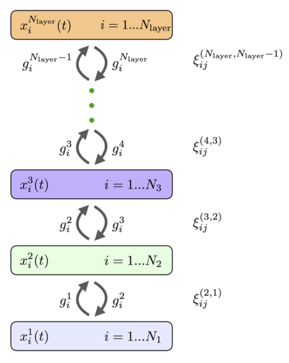
The neurons can be organized in layers so that every neuron in a given layer has the same activation function and the same dynamic time scale. If we assume that there are no horizontal connections between the neurons within the layer (lateral connections) and there are no skip-layer connections, the general fully connected network (11), (12) reduces to the architecture shown in Fig.4. It has [math]\displaystyle{ N_\text{layer} }[/math] layers of recurrently connected neurons with the states described by continuous variables [math]\displaystyle{ x_i^{A} }[/math] and the activation functions [math]\displaystyle{ g_i^{A} }[/math], index [math]\displaystyle{ A }[/math] enumerates the layers of the network, and index [math]\displaystyle{ i }[/math] enumerates individual neurons in that layer. The activation functions can depend on the activities of all the neurons in the layer. Every layer can have a different number of neurons [math]\displaystyle{ N_A }[/math]. These neurons are recurrently connected with the neurons in the preceding and the subsequent layers. The matrices of weights that connect neurons in layers [math]\displaystyle{ A }[/math] and [math]\displaystyle{ B }[/math] are denoted by [math]\displaystyle{ \xi^{(A,B)}_{ij} }[/math] (the order of the upper indices for weights is the same as the order of the lower indices, in the example above this means that the index [math]\displaystyle{ i }[/math] enumerates neurons in the layer [math]\displaystyle{ A }[/math], and index [math]\displaystyle{ j }[/math] enumerates neurons in the layer [math]\displaystyle{ B }[/math]). The feedforward weights and the feedback weights are equal. The dynamical equations for the neurons' states can be written as

[math]\displaystyle{ \tau_A \frac{dx_i^A}{dt} = \sum\limits_{j=1}^{N_{A-1}} \xi^{(A, A-1)}_{ij} g_j^{A-1} + \sum\limits_{j=1}^{N_{A+1}} \xi^{(A, A+1)}_{ij} g_j^{A+1} - x_i^A }[/math]

(14)

with boundary conditions

[math]\displaystyle{ g_i^0 =0, \ \ \ \ \ \text{and}\ \ \ \ \ g_i^{N_\text{layer}+1}=0 }[/math]

(15)

The main difference of these equations from the conventional feedforward networks is the presence of the second term, which is responsible for the feedback from higher layers. These top-down signals help neurons in lower layers to decide on their response to the presented stimuli. Following the general recipe it is convenient to introduce a Lagrangian function [math]\displaystyle{ L^A(\{x^A_i\}) }[/math] for the [math]\displaystyle{ A }[/math]-th hidden layer, which depends on the activities of all the neurons in that layer. The activation functions in that layer can be defined as partial derivatives of the Lagrangian

[math]\displaystyle{ g_i^A = \frac{\partial L^A}{\partial x_i^A} }[/math]

(16)

With these definitions the energy (Lyapunov) function is given by

[math]\displaystyle{ E = \sum\limits_{A=1}^{N_\text{layer}} \Big[ \sum\limits_{i=1}^{N_A} x_i^A g_i^A - L^{A}\Big] - \sum\limits_{A=1}^{N_\text{layer}-1} \sum\limits_{i=1}^{N_{A+1}} \sum\limits_{j=1}^{N_A} g_i^{A+1} \xi^{(A+1,A)}_{ij} g_j^A }[/math]

(17)

If the Lagrangian functions, or equivalently the activation functions, are chosen in such a way that the Hessians for each layer are positive semi-definite and the overall energy is bounded from below, this system is guaranteed to converge to a fixed point attractor state. The temporal derivative of this energy function is given by

[math]\displaystyle{ \frac{dE}{dt} = -\sum\limits_{A=1}^{N_\text{layer}} \tau_A \sum\limits_{i,j=1}^{N_A} \frac{dx_j^A}{dt} \frac{\partial^2 L^{A}}{\partial x_j^{A} \partial x_i^{A}} \frac{dx_i^A}{dt} \leq 0 }[/math]

(18)

Thus, the hierarchical layered network is indeed an attractor network with the global energy function. This network is described by a hierarchical set of synaptic weights that can be learned for each specific problem.

References

- ↑ 1.0 1.1 1.2 1.3 1.4 1.5 1.6 Hopfield, John (1982). "Neural networks and physical systems with emergent collective computational abilities". Proceedings of the National Academy of Sciences 79 (8): 2554–2558. doi:10.1073/pnas.79.8.2554. PMID 6953413.
- ↑ 2.0 2.1 Hopfield, John (1984). "Neurons with graded response have collective computational properties like those of two-state neurons". Proceedings of the National Academy of Sciences 81 (10): 3088–3092. doi:10.1073/pnas.81.10.3088. PMID 6587342.
- ↑ 3.0 3.1 3.2 3.3 3.4 3.5 3.6 Krotov, Dmitry; Hopfield, John (2016). "Dense Associative Memory for Pattern Recognition". Neural Information Processing Systems 29: 1172–1180.
- ↑ 4.0 4.1 4.2 4.3 Ramsauer, Hubert et al. (2021). "Hopfield Networks is All You Need". International Conference on Learning Representations.
- ↑ 5.0 5.1 5.2 Demircigil, Mete et al. (2017). "On a model of associative memory with huge storage capacity.". Journal of Statistical Physics 168 (2): 288–299. doi:10.1007/s10955-017-1806-y. https://link.springer.com/article/10.1007/s10955-017-1806-y.
- ↑ 6.00 6.01 6.02 6.03 6.04 6.05 6.06 6.07 6.08 6.09 Krotov, Dmitry; Hopfield, John (2021). "Large associative memory problem in neurobiology and machine learning.". International Conference on Learning Representations.
- ↑ 7.0 7.1 7.2 7.3 7.4 7.5 7.6 7.7 7.8 Krotov, Dmitry (2021). "Hierarchical Associative Memory". arXiv:2107.06446 [cs.NE].
This article needs additional or more specific categories. (August 2021) |