Moving horizon estimation
Moving horizon estimation (MHE) is an optimization approach that uses a series of measurements observed over time, containing noise (random variations) and other inaccuracies, and produces estimates of unknown variables or parameters. Unlike deterministic approaches, MHE requires an iterative approach that relies on linear programming or nonlinear programming solvers to find a solution.[1] MHE reduces to the Kalman filter under certain simplifying conditions.[2] A critical evaluation of the extended Kalman filter and the MHE found that the MHE improved performance at the cost of increased computational expense.[3] Because of the computational expense, MHE has generally been applied to systems where there are greater computational resources and moderate to slow system dynamics. However, in the literature there are some methods to accelerate this method.[4][5]
Overview
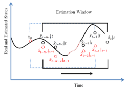
The application of MHE is generally to estimate measured or unmeasured states of dynamical systems. Initial conditions and parameters within a model are adjusted by MHE to align measured and predicted values. MHE is based on a finite horizon optimization of a process model and measurements. At time t the current process state is sampled and a minimizing strategy is computed (via a numerical minimization algorithm) for a relatively short time horizon in the past: . Specifically, an online or on-the-fly calculation is used to explore state trajectories that find (via the solution of Euler–Lagrange equations) an objective-minimizing strategy until time . Only the last step of the estimation strategy is used, then the process state is sampled again and the calculations are repeated starting from the time-shifted states, yielding a new state path and predicted parameters. The estimation horizon keeps being shifted forward and for this reason the technique is called moving horizon estimation. Although this approach is not optimal, in practice it has given very good results when compared with the Kalman filter and other estimation strategies.
Principles of MHE
Moving horizon estimation (MHE) is a multivariable estimation algorithm that uses:
- an internal dynamic model of the process
- a history of past measurements and
- an optimization cost function J over the estimation horizon,
to calculate the optimum states and parameters.

The optimization estimation function is given by:
without violating state or parameter constraints (low/high limits)
With:
= i -th model predicted variable (e.g. predicted temperature)
= i -th measured variable (e.g. measured temperature)
= i -th estimated parameter (e.g. heat transfer coefficient)
= weighting coefficient reflecting the relative importance of measured values
= weighting coefficient reflecting the relative importance of prior model predictions
= weighting coefficient penalizing relative big changes in
Moving horizon estimation uses a sliding time window. At each sampling time the window moves one step forward. It estimates the states in the window by analyzing the measured output sequence and uses the last estimated state out of the window, as the prior knowledge.
Applications
- MATLAB, Python, and Simulink source code for MHE: Python, MATLAB, and Simulink CSTR Example
- Monitoring of industrial process fouling [6]
- Oil and gas industry [7]
- Polymer manufacture[8]
- Unmanned aerial systems[9][10]
See also
- Alpha beta filter
- Data assimilation
- Ensemble Kalman filter
- Extended Kalman filter
- Invariant extended Kalman filter
- Fast Kalman filter
- Filtering problem (stochastic processes)
- Kernel adaptive filter
- Non-linear filter
- Particle filter
- Predictor corrector
- Recursive least squares
- Schmidt–Kalman filter
- Sliding mode control
- Wiener filter
References
- ↑ J.D. Hedengren; R. Asgharzadeh Shishavan; K.M. Powell; T.F. Edgar (2014). "Nonlinear modeling, estimation and predictive control in APMonitor". Computers & Chemical Engineering 70 (5): 133–148. doi:10.1016/j.compchemeng.2014.04.013. https://scholarsarchive.byu.edu/facpub/1667.
- ↑ Rao, C.V.; Rawlings, J.B.; Maynes, D.Q (2003). "Constrained State Estimation for Nonlinear Discrete-Time Systems: Stability and Moving Horizon Approximations". IEEE Transactions on Automatic Control 48 (2): 246–258. doi:10.1109/tac.2002.808470.
- ↑ Haseltine, E.J.; Rawlings, J.B. (2005). "Critical Evaluation of Extended Kalman Filtering and Moving-Horizon Estimation". Ind. Eng. Chem. Res. 44 (8): 2451–2460. doi:10.1021/ie034308l. http://pubs.acs.org/cgi-bin/abstract.cgi/iecred/2005/44/i08/abs/ie034308l.html.
- ↑ 4.0 4.1 Hashemian, N.; Armaou, A. (2015). "Fast Moving Horizon Estimation of nonlinear processes via Carleman linearization". 2015 American Control Conference (ACC). pp. 3379–3385. doi:10.1109/ACC.2015.7171854. ISBN 978-1-4799-8684-2.
- ↑ Hashemian, N.; Armaou, A. (2016). "Simulation, model-reduction and state estimation of a two-component coagulation process". AIChE Journal 62 (5): 1557–1567. doi:10.1002/aic.15146.
- ↑ Spivey, B.; Hedengren, J. D.; Edgar, T. F. (2010). "Constrained Nonlinear Estimation for Industrial Process Fouling". Industrial & Engineering Chemistry Research 49 (17): 7824–7831. doi:10.1021/ie9018116.
- ↑ Hedengren, J.D. (2012). Advanced Process Monitoring. Springer’s International Series in Operations Research and Management Science. http://prism.groups.et.byu.net/uploads/Members/hedengren_apm2012.pdf. Retrieved 2012-09-18.
- ↑ Ramlal, J. (2007). "Moving Horizon Estimation for an Industrial Gas Phase Polymerization Reactor". IFAC Symposium on Nonlinear Control Systems Design (NOLCOS). Archived from the original on 2009-09-20. https://web.archive.org/web/20090920070424/http://apmonitor.com/Documents/mhe.pdf.
- ↑ Sun, L. (2013). "Optimal Trajectory Generation using Model Predictive Control for Aerially Towed Cable Systems". Journal of Guidance, Control, and Dynamics 37 (2): 525. doi:10.2514/1.60820. Bibcode: 2014JGCD...37..525S. http://apm.byu.edu/prism/uploads/Members/sun_2013.pdf.
- ↑ Sun, L. (2015). "Parameter Estimation for Towed Cable Systems Using Moving Horizon Estimation". IEEE Transactions on Aerospace and Electronic Systems 51 (2): 1432–1446. doi:10.1109/TAES.2014.130642. Bibcode: 2015ITAES..51.1432S. http://apm.byu.edu/prism/uploads/Members/SunCastagnoHedengren14.pdf.
Further reading
- Rawlings, James B. (2009). Model Predictive Control: Theory and Design. Mathematics in Science and Engineering. Madison, WI: Nob Hill Publishing, LLC. pp. 576. ISBN 978-0-9759377-0-9.
External links
- MHE with Python GEKKO
- MHE Tutorial in Simulink and MATLAB
- MHE lecture material
- Online Course: MHE in Simulink, MATLAB and Python
 |
