Non-parametric methods in statistics
Methods in mathematical statistics that do not assume a knowledge of the functional form of general distributions. The name "non-parametric method" emphasizes their contrast to the classical, parametric, methods, in which it is assumed that the general distribution is known up to finitely many parameters, and which make it possible to estimate the unknown values of these parameters from results of observations and to test hypotheses concerning their values.
Example. Let <img align="absmiddle" border="0" src="https://www.encyclopediaofmath.org/legacyimages/n/n067/n067230/n0672301.png" /> and <img align="absmiddle" border="0" src="https://www.encyclopediaofmath.org/legacyimages/n/n067/n067230/n0672302.png" /> be two independent samples derived from populations with continuous general distribution functions <img align="absmiddle" border="0" src="https://www.encyclopediaofmath.org/legacyimages/n/n067/n067230/n0672303.png" /> and <img align="absmiddle" border="0" src="https://www.encyclopediaofmath.org/legacyimages/n/n067/n067230/n0672304.png" />; suppose that the hypothesis <img align="absmiddle" border="0" src="https://www.encyclopediaofmath.org/legacyimages/n/n067/n067230/n0672305.png" /> that <img align="absmiddle" border="0" src="https://www.encyclopediaofmath.org/legacyimages/n/n067/n067230/n0672306.png" /> and <img align="absmiddle" border="0" src="https://www.encyclopediaofmath.org/legacyimages/n/n067/n067230/n0672307.png" /> are equal is to be tested against the alternative of a shift, that is, the hypothesis
| <img align="absmiddle" border="0" src="https://www.encyclopediaofmath.org/legacyimages/n/n067/n067230/n0672308.png" /> |
for all <img align="absmiddle" border="0" src="https://www.encyclopediaofmath.org/legacyimages/n/n067/n067230/n0672309.png" /> and some <img align="absmiddle" border="0" src="https://www.encyclopediaofmath.org/legacyimages/n/n067/n067230/n06723010.png" />. In the classical version it is assumed that <img align="absmiddle" border="0" src="https://www.encyclopediaofmath.org/legacyimages/n/n067/n067230/n06723011.png" /> and <img align="absmiddle" border="0" src="https://www.encyclopediaofmath.org/legacyimages/n/n067/n067230/n06723012.png" /> are normal distribution functions, and to test the hypothesis in question one uses the Student test. In the non-parametric statement of the problem no assumptions are made on the form of <img align="absmiddle" border="0" src="https://www.encyclopediaofmath.org/legacyimages/n/n067/n067230/n06723013.png" /> and <img align="absmiddle" border="0" src="https://www.encyclopediaofmath.org/legacyimages/n/n067/n067230/n06723014.png" /> except continuity. A typical non-parametric test for testing the hypothesis <img align="absmiddle" border="0" src="https://www.encyclopediaofmath.org/legacyimages/n/n067/n067230/n06723015.png" /> against <img align="absmiddle" border="0" src="https://www.encyclopediaofmath.org/legacyimages/n/n067/n067230/n06723016.png" /> is the Wilcoxon test, which is based on the sum of the ranks of the first sample in the series of joint order statistics. One rejects the hypothesis that the distributions are equal if the test statistic computed from the observations turns out to be too large or too small. The statistic of Wilcoxon's test is easy to calculate and its distribution under <img align="absmiddle" border="0" src="https://www.encyclopediaofmath.org/legacyimages/n/n067/n067230/n06723017.png" /> does not depend on <img align="absmiddle" border="0" src="https://www.encyclopediaofmath.org/legacyimages/n/n067/n067230/n06723018.png" />. The critical values corresponding to a given significance level for small values of <img align="absmiddle" border="0" src="https://www.encyclopediaofmath.org/legacyimages/n/n067/n067230/n06723019.png" /> and <img align="absmiddle" border="0" src="https://www.encyclopediaofmath.org/legacyimages/n/n067/n067230/n06723020.png" /> can be found in tables (see, for example, [1]); for large <img align="absmiddle" border="0" src="https://www.encyclopediaofmath.org/legacyimages/n/n067/n067230/n06723021.png" /> and <img align="absmiddle" border="0" src="https://www.encyclopediaofmath.org/legacyimages/n/n067/n067230/n06723022.png" /> one uses a normal approximation.
In a number of cases it is important not only to test the hypothesis of absence of a shift, but also to estimate this shift <img align="absmiddle" border="0" src="https://www.encyclopediaofmath.org/legacyimages/n/n067/n067230/n06723023.png" />, which can be interpreted, for example, as the change in yield when a method of tilling the land is replaced by another, or as the additional time of sleep after taking a pill. The estimate of the parameter <img align="absmiddle" border="0" src="https://www.encyclopediaofmath.org/legacyimages/n/n067/n067230/n06723024.png" /> given by the quantity <img align="absmiddle" border="0" src="https://www.encyclopediaofmath.org/legacyimages/n/n067/n067230/n06723025.png" />, which is quite satisfactory in the normal case, may be very unsuitable under departures from normality and may be even inconsistent. A non-parametric estimate of <img align="absmiddle" border="0" src="https://www.encyclopediaofmath.org/legacyimages/n/n067/n067230/n06723026.png" /> may enjoy vastly better properties in this respect (see [2]); for example, the median of the collection of <img align="absmiddle" border="0" src="https://www.encyclopediaofmath.org/legacyimages/n/n067/n067230/n06723027.png" /> numbers <img align="absmiddle" border="0" src="https://www.encyclopediaofmath.org/legacyimages/n/n067/n067230/n06723028.png" />, <img align="absmiddle" border="0" src="https://www.encyclopediaofmath.org/legacyimages/n/n067/n067230/n06723029.png" />, <img align="absmiddle" border="0" src="https://www.encyclopediaofmath.org/legacyimages/n/n067/n067230/n06723030.png" />. This estimate is closely connected with the Wilcoxon test. One could say that it stands in the same relation to the estimate <img align="absmiddle" border="0" src="https://www.encyclopediaofmath.org/legacyimages/n/n067/n067230/n06723031.png" /> as the Wilcoxon test to the Student test.
Notwithstanding the great variety of problems that can be solved by non-parametric methods, these problems can conventionally be divided into two large parts: problems of testing hypotheses and problems of estimating unknown distributions and parameters, which are understood as certain functionals of these distributions.
Non-parametric testing of statistical hypotheses is the most generally developed part of non-parametric methods in statistics. It is required to set up a procedure (a test) that makes it possible to accept or reject the hypothesis to be tested against a given alternative. A typical example is the goodness-of-fit test, and other important examples for applications are tests for symmetry, independence and randomness.
The problem of testing goodness-of-fit consists in the following: From a sample of a population with general distribution function <img align="absmiddle" border="0" src="https://www.encyclopediaofmath.org/legacyimages/n/n067/n067230/n06723032.png" /> one has to test the hypothesis <img align="absmiddle" border="0" src="https://www.encyclopediaofmath.org/legacyimages/n/n067/n067230/n06723033.png" />, where <img align="absmiddle" border="0" src="https://www.encyclopediaofmath.org/legacyimages/n/n067/n067230/n06723034.png" /> is a given continuous distribution function. The non-parametric nature of the problem manifests itself here in the non-parametric alternative, which can be stated, for example, in a one-sided: <img align="absmiddle" border="0" src="https://www.encyclopediaofmath.org/legacyimages/n/n067/n067230/n06723035.png" /> or <img align="absmiddle" border="0" src="https://www.encyclopediaofmath.org/legacyimages/n/n067/n067230/n06723036.png" />, or two-sided version: <img align="absmiddle" border="0" src="https://www.encyclopediaofmath.org/legacyimages/n/n067/n067230/n06723037.png" />.
The problem of testing symmetry consists in testing the symmetry of a general distribution function <img align="absmiddle" border="0" src="https://www.encyclopediaofmath.org/legacyimages/n/n067/n067230/n06723038.png" /> relative to a given point <img align="absmiddle" border="0" src="https://www.encyclopediaofmath.org/legacyimages/n/n067/n067230/n06723039.png" />, that is,
| <img align="absmiddle" border="0" src="https://www.encyclopediaofmath.org/legacyimages/n/n067/n067230/n06723040.png" /> |
As alternative one can take one-sided conditions
| <img align="absmiddle" border="0" src="https://www.encyclopediaofmath.org/legacyimages/n/n067/n067230/n06723041.png" /> |
| <img align="absmiddle" border="0" src="https://www.encyclopediaofmath.org/legacyimages/n/n067/n067230/n06723042.png" /> |
with strict inequality for at least one <img align="absmiddle" border="0" src="https://www.encyclopediaofmath.org/legacyimages/n/n067/n067230/n06723043.png" />, or two-sided conditions of the same type.
The problem of testing independence arises in cases when one has to decide whether two characteristics observed in one and the same object are independent, given independent observations on these objects.
In a similar fashion one can state the hypothesis of randomness, when it is assumed that the elements of a sample are independent identically-distributed quantities. Apart from alternatives of a general form there also occur cases when it turns out to be possible to indicate in precisely what way the distributions of the elements of a sample differ under an alternative; in this way, for example, the alternatives of trend and regression arise.
Methods of algorithmic construction of non-parametric procedures with given properties have so far only been worked out inadequately, and as a rule, intuition and heuristic arguments play a major role in the choice of a suitable procedure. In this way a large body of methods and devices for solving frequently occurring non-parametric problems has been accumulated (see [3]).
An extensive group of non-parametric tests is based on the use of empirical distribution functions. Let <img align="absmiddle" border="0" src="https://www.encyclopediaofmath.org/legacyimages/n/n067/n067230/n06723044.png" /> be an empirical distribution function constructed from a sample of size <img align="absmiddle" border="0" src="https://www.encyclopediaofmath.org/legacyimages/n/n067/n067230/n06723045.png" /> in a population with general distribution function <img align="absmiddle" border="0" src="https://www.encyclopediaofmath.org/legacyimages/n/n067/n067230/n06723046.png" />. By the Glivenko–Cantelli theorem,
| <img align="absmiddle" border="0" src="https://www.encyclopediaofmath.org/legacyimages/n/n067/n067230/n06723047.png" /> |
with probability 1. Thus, the empirical and true distribution functions uniformly approach each other with probability 1 and one can base tests for goodness-of-fit with an hypothesis on the true distribution function on measures of their proximity.
The first tests of this kind were the Kolmogorov test and the Cramér–von Mises test, which were put forward at the beginning of the 1930's and were based, respectively, on the statistics
| <img align="absmiddle" border="0" src="https://www.encyclopediaofmath.org/legacyimages/n/n067/n067230/n06723048.png" /> |
and
| <img align="absmiddle" border="0" src="https://www.encyclopediaofmath.org/legacyimages/n/n067/n067230/n06723049.png" /> |
It should be mentioned that both these statistics have distributions that are independent of the general distribution function <img align="absmiddle" border="0" src="https://www.encyclopediaofmath.org/legacyimages/n/n067/n067230/n06723050.png" />, provided only that the latter is continuous. Their limiting distributions, which were found in the middle of the 1930's by A.N. Kolmogorov and N.N. Smirnov, have been tabulated, which makes it possible to find the boundary of the critical domain corresponding to a given significance level.
Many versions of tests for goodness-of-fit based on the difference between <img align="absmiddle" border="0" src="https://www.encyclopediaofmath.org/legacyimages/n/n067/n067230/n06723051.png" /> and <img align="absmiddle" border="0" src="https://www.encyclopediaofmath.org/legacyimages/n/n067/n067230/n06723052.png" /> have been proposed and studied, for example the Rényi test and the tests of Anderson–Darling, Watson and others (see [4]). For a successful application in the case of large samples one has to know the relevant limiting distributions in the first instance. They can be found by an approach according to which the test statistic is presented as a continuous functional of an empirical process,
| <img align="absmiddle" border="0" src="https://www.encyclopediaofmath.org/legacyimages/n/n067/n067230/n06723053.png" /> |
where <img align="absmiddle" border="0" src="https://www.encyclopediaofmath.org/legacyimages/n/n067/n067230/n06723054.png" /> is an empirical distribution function constructed from a sample of size <img align="absmiddle" border="0" src="https://www.encyclopediaofmath.org/legacyimages/n/n067/n067230/n06723055.png" /> of a uniform distribution on <img align="absmiddle" border="0" src="https://www.encyclopediaofmath.org/legacyimages/n/n067/n067230/n06723056.png" />. The process <img align="absmiddle" border="0" src="https://www.encyclopediaofmath.org/legacyimages/n/n067/n067230/n06723057.png" /> converges weakly in the space <img align="absmiddle" border="0" src="https://www.encyclopediaofmath.org/legacyimages/n/n067/n067230/n06723058.png" /> to a Gaussian process, a so-called Brownian bridge (cf. [6]). Therefore the limiting distribution of the studied statistic coincides with the distribution of the corresponding functional on the Brownian bridge, which can be computed by standard methods.
There are modifications of the statistics <img align="absmiddle" border="0" src="https://www.encyclopediaofmath.org/legacyimages/n/n067/n067230/n06723059.png" /> and <img align="absmiddle" border="0" src="https://www.encyclopediaofmath.org/legacyimages/n/n067/n067230/n06723060.png" /> that are intended to test hypotheses on the distribution in the multi-dimensional case and also to test hypotheses of independence and symmetry. In these cases a number of additional difficulties arise. For example, in the multi-dimensional case all the statistics in question cease to have the property of universality (independence of the original distribution). Most important is the case of a uniform distribution on the unit cube, because a sample for a multi-dimensional distribution can in one way or another be transformed into a sample from a uniform distribution. However, neither the exact nor the limiting distributions of the Kolmogorov statistic are known (1982), not even in this simple case. Similar difficulties emerge when one has to test not a simple, but a composite hypothesis on the distribution, that is, when one assumes that the general distribution function is of the form <img align="absmiddle" border="0" src="https://www.encyclopediaofmath.org/legacyimages/n/n067/n067230/n06723061.png" />, where <img align="absmiddle" border="0" src="https://www.encyclopediaofmath.org/legacyimages/n/n067/n067230/n06723062.png" /> is an unknown one- or multi-dimensional parameter. In this case it is natural to estimate <img align="absmiddle" border="0" src="https://www.encyclopediaofmath.org/legacyimages/n/n067/n067230/n06723063.png" /> from a sample, for example, by a maximum-likelihood estimator <img align="absmiddle" border="0" src="https://www.encyclopediaofmath.org/legacyimages/n/n067/n067230/n06723064.png" /> (cf. Maximum-likelihood method), and to compare <img align="absmiddle" border="0" src="https://www.encyclopediaofmath.org/legacyimages/n/n067/n067230/n06723065.png" /> with <img align="absmiddle" border="0" src="https://www.encyclopediaofmath.org/legacyimages/n/n067/n067230/n06723066.png" />. The statistics <img align="absmiddle" border="0" src="https://www.encyclopediaofmath.org/legacyimages/n/n067/n067230/n06723067.png" />, <img align="absmiddle" border="0" src="https://www.encyclopediaofmath.org/legacyimages/n/n067/n067230/n06723068.png" /> and their modifications can be constructed as in the case of a simple hypothesis. However, the distributions of these statistics, both exact and limiting, turn out again to depend on the form of <img align="absmiddle" border="0" src="https://www.encyclopediaofmath.org/legacyimages/n/n067/n067230/n06723069.png" /> and in many cases also on the unknown true value of <img align="absmiddle" border="0" src="https://www.encyclopediaofmath.org/legacyimages/n/n067/n067230/n06723070.png" />. The task of computing these distributions is tedious, and their exact form is not known, although for statistics like <img align="absmiddle" border="0" src="https://www.encyclopediaofmath.org/legacyimages/n/n067/n067230/n06723071.png" /> tables of limiting distribution have been set up in a number of cases (see [5]). For some other statistics simulated percentage points are known.
Apart from the goodness-of-fit tests considered, their two-sample and multi-sample analogues have also been constructed, which can be used to test goodness-of-fit as well as homogeneity of certain samples (see Smirnov test).
A common property of tests for goodness-of-fit and uniformity based on empirical distribution functions is their consistency against arbitrary alternatives. However, the choice of one statistic or another in a practical problem is hampered because their powers are insufficiently studied. For samples of large size one can rely on a knowledge of the Pitman asymptotic relative efficiency, which has been computed for a number of the simplest statistics (see [7]).
Rank tests form another group of non-parametric tests (cf. Rank test). The earliest use of the rank sign test occurs in the work of J. Arbuthnott (1710), who used it to analyze statistical data on the birth-rate of boys and girls to obtain "arguments for divine providence" . But the modern period of development of rank tests begins at the end of the 1930's. After the publication in 1945 of F. Wilcoxon's paper, in which he proposed the rank test bearing his name (cf. Wilcoxon test), rank methods entered into a period of intense development.
The use of rank procedures is based on the following arguments. Since the rank vector together with the vector of order statistics contains the entire information embodied in the sample, a certain part of the information is contained in the rank vector only. One can construct statistical procedures based only on the ranks without using knowledge of the sample values themselves. The advantage of such procedures is their computational simplicity, which follows from the fact that the ranks are integers. Another important feature of rank procedures is their advantage in cases when the observations are of a qualitative, not quantitative, nature, as long as they admit an ordering, which is practically important in research in sociology, psychology and medicine. Finally, the distributions of rank statistics under the null hypotheses do not depend on the underlying distribution, which makes it possible to compute these distributions once and for all.
As rank methods developed it became clear that the part of the information contained in the rank vector can prove to be significant, in which case these procedures are highly efficient. In the example studied above, connected with testing homogeneity of two samples, an extension of the domain of applicability of the test leads to a loss in power, and in the normal case Student's test (cf. Student test) is more powerful than any rank test. However, when there is a large number of observations, Wilcoxon's test loses little compared with Student's test. It turns out that in the normal case the asymptotic relative efficiency of Wilcoxon's test to Student's test is <img align="absmiddle" border="0" src="https://www.encyclopediaofmath.org/legacyimages/n/n067/n067230/n06723072.png" />. But when the underlying distribution differs from the normal one, then the asymptotic relative efficiency in question can be arbitrarily large, but never drops below 0.864 (see [4]). Moreover, there is a rank test (the so-called normal scores test) with asymptotic relative efficiency 1 relative to Student's test in the normal case and exceeding 1 for any deviation from normality. Thus, this test turns out to be asymptotically preferable to Student's test.
Another example is connected with testing the hypothesis of symmetry. Suppose that a sample <img align="absmiddle" border="0" src="https://www.encyclopediaofmath.org/legacyimages/n/n067/n067230/n06723073.png" /> is extracted from a population with general density <img align="absmiddle" border="0" src="https://www.encyclopediaofmath.org/legacyimages/n/n067/n067230/n06723074.png" /> and that one wishes to test the hypothesis that <img align="absmiddle" border="0" src="https://www.encyclopediaofmath.org/legacyimages/n/n067/n067230/n06723075.png" /> is symmetric with respect to zero, again with the alternative of a shift. The simplest test in this case is the sign test, which is based on the number of positive values among the <img align="absmiddle" border="0" src="https://www.encyclopediaofmath.org/legacyimages/n/n067/n067230/n06723076.png" />. Wilcoxon's signed rank test is based on the statistic <img align="absmiddle" border="0" src="https://www.encyclopediaofmath.org/legacyimages/n/n067/n067230/n06723077.png" />, where <img align="absmiddle" border="0" src="https://www.encyclopediaofmath.org/legacyimages/n/n067/n067230/n06723078.png" /> is the rank of <img align="absmiddle" border="0" src="https://www.encyclopediaofmath.org/legacyimages/n/n067/n067230/n06723079.png" /> in the series of order statistics for <img align="absmiddle" border="0" src="https://www.encyclopediaofmath.org/legacyimages/n/n067/n067230/n06723080.png" />. The statistic of this test uses not only the information about the signs of the observations but also about their magnitude. Therefore, one can expect that Wilcoxon's test will be more efficient than the sign test. Actually, the asymptotic relative efficiency of these tests to Student's test are <img align="absmiddle" border="0" src="https://www.encyclopediaofmath.org/legacyimages/n/n067/n067230/n06723081.png" /> and <img align="absmiddle" border="0" src="https://www.encyclopediaofmath.org/legacyimages/n/n067/n067230/n06723082.png" /> (in the normal case). Thus, Wilcoxon's test exceeds the sign test by a factor of <img align="absmiddle" border="0" src="https://www.encyclopediaofmath.org/legacyimages/n/n067/n067230/n06723083.png" /> and concedes little to Student's test.
Another example is connected with testing the hypothesis of independence. Suppose that there is a number of objects each of which has two attributes, quantitative or qualitative (the mathematical and musical talents of a student, the colour and the ripeness of berries, etc.). It is assumed that observations on the quantitative attributes can be ordered. It is required to test from <img align="absmiddle" border="0" src="https://www.encyclopediaofmath.org/legacyimages/n/n067/n067230/n06723084.png" /> independent observations on the objects, the hypothesis that the attributes are independent against the alternative, say, that they are positively dependent. Let <img align="absmiddle" border="0" src="https://www.encyclopediaofmath.org/legacyimages/n/n067/n067230/n06723085.png" /> and <img align="absmiddle" border="0" src="https://www.encyclopediaofmath.org/legacyimages/n/n067/n067230/n06723086.png" /> be the ranks of the attributes corresponding to the <img align="absmiddle" border="0" src="https://www.encyclopediaofmath.org/legacyimages/n/n067/n067230/n06723087.png" />-th observation. A natural criterion to test independence is Spearman's coefficient of rank correlation <img align="absmiddle" border="0" src="https://www.encyclopediaofmath.org/legacyimages/n/n067/n067230/n06723088.png" />, which can be computed by the formula
| <img align="absmiddle" border="0" src="https://www.encyclopediaofmath.org/legacyimages/n/n067/n067230/n06723089.png" /> |
The hypothesis of independence is rejected for large values of <img align="absmiddle" border="0" src="https://www.encyclopediaofmath.org/legacyimages/n/n067/n067230/n06723090.png" />, i.e. close to 1.
The critical values for small <img align="absmiddle" border="0" src="https://www.encyclopediaofmath.org/legacyimages/n/n067/n067230/n06723091.png" /> can be found in tables; for large <img align="absmiddle" border="0" src="https://www.encyclopediaofmath.org/legacyimages/n/n067/n067230/n06723092.png" /> one uses a normal approximation. The asymptotic relative efficiency of the test based on <img align="absmiddle" border="0" src="https://www.encyclopediaofmath.org/legacyimages/n/n067/n067230/n06723093.png" /> relative to that based on the sampling correlation coefficient is again fairly high, namely <img align="absmiddle" border="0" src="https://www.encyclopediaofmath.org/legacyimages/n/n067/n067230/n06723094.png" /> in the normal case (see [9]).
Since for the testing of each non-parametric hypothesis there are many rank tests, frequently proposed from heuristic arguments, the choice must be based on certain optimality arguments. As is known, uniformly most-powerful tests in the class of all possible alternatives rarely exist, even in the parametric case. Therefore, by optimal rank tests for finite sample sizes one means just locally most-powerful tests. For example, Wilcoxon's test is locally most powerful in the two-sample problem of testing homogeneity against the alternative of a shift for the logistic distribution with density <img align="absmiddle" border="0" src="https://www.encyclopediaofmath.org/legacyimages/n/n067/n067230/n06723095.png" />, and the normal scores test in the same problem for a normal distribution. In the asymptotic theory for the corresponding property of optimality one uses a certain concept of asymptotic efficiency, and locally most-powerful tests usually turn out to be asymptotically optimal (see [8]).
In the theory of rank tests it is assumed that the distributions of the observations are continuous, so that they can be ordered without ties and the rank statistics are uniquely determined. However, in practice observations are always rounded-off, therefore ties sometimes appear. The following two methods are most commonly used for overcoming this difficulty. The first one consists in randomly ordering tied observations. In the second method one assigns the average rank of the group to each of a group of tied observations. The merits of the two methods have not yet been sufficiently investigated.
Non-parametric estimation is a section of non-parametric statistics that deals with problems of estimating unknown distributions or functions of them such as quantiles, moments, modes, entropy, information in the sense of Fisher, etc.
The most widely used estimator for an unknown distribution function is the empirical one. The strong uniform consistency of it as an estimator of an unknown distribution function follows from the Glivenko–Cantelli theorem, and its minimax character has been established in [10]. But consistent estimation of an unknown density is a more complicated problem. For the estimation problem to be well-posed, additional a priori information is needed on the class <img align="absmiddle" border="0" src="https://www.encyclopediaofmath.org/legacyimages/n/n067/n067230/n06723096.png" /> of densities to which the relevant density <img align="absmiddle" border="0" src="https://www.encyclopediaofmath.org/legacyimages/n/n067/n067230/n06723097.png" /> belongs. In the classical statements the a priori family of densities is given in parametric form and is determined by a finite-dimensional vector of the unknown parameters. In the non-parametric statement the problem assumes an infinite-dimensional character, and the accuracy of the estimation of an unknown density depends essentially (cf. [11]) on a geometric characterization of the "massiveness" of the class <img align="absmiddle" border="0" src="https://www.encyclopediaofmath.org/legacyimages/n/n067/n067230/n06723098.png" />.
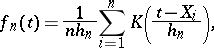
The most extensively used estimators of an unknown density <img align="absmiddle" border="0" src="https://www.encyclopediaofmath.org/legacyimages/n/n067/n067230/n06723099.png" /> are "kernel estimators"
| <img align="absmiddle" border="0" src="https://www.encyclopediaofmath.org/legacyimages/n/n067/n067230/n067230100.png" /> |
where the <img align="absmiddle" border="0" src="https://www.encyclopediaofmath.org/legacyimages/n/n067/n067230/n067230101.png" /> are observations, the kernel function <img align="absmiddle" border="0" src="https://www.encyclopediaofmath.org/legacyimages/n/n067/n067230/n067230102.png" /> is absolutely integrable and satisfies the condition
| <img align="absmiddle" border="0" src="https://www.encyclopediaofmath.org/legacyimages/n/n067/n067230/n067230103.png" /> |
and the sequence <img align="absmiddle" border="0" src="https://www.encyclopediaofmath.org/legacyimages/n/n067/n067230/n067230104.png" /> is such that <img align="absmiddle" border="0" src="https://www.encyclopediaofmath.org/legacyimages/n/n067/n067230/n067230105.png" /> as <img align="absmiddle" border="0" src="https://www.encyclopediaofmath.org/legacyimages/n/n067/n067230/n067230106.png" />. In some cases one uses other non-parametric estimators of the density: simpler ones (the histogram, the frequency polygon) or more complicated ones, for example, Chentsov's projection estimators. The question of the accuracy of approximation by these estimators to an unknown density in relation to properties of the class <img align="absmiddle" border="0" src="https://www.encyclopediaofmath.org/legacyimages/n/n067/n067230/n067230107.png" /> has been well studied (see [11], [12]).
An empirical distribution function and a non-parametric estimator of the density can be used to estimate functionals of unknown general distributions; for this purpose it is sufficient to replace the unknown distribution by its estimators in the expressions for the functional in question. The idea itself and the beginning of its realization go back to work of R. von Mises in the 1930's and 1940's. It has been proved that under certain restrictions on the class of functions to be estimated and on the non-parametric class of distributions there exists a minimax lower bound on the quality of non-parametric estimators (see [12]). Non-parametric estimation is closely connected with the problem of constructing robust estimates.
References
| [1] | L.N. Bol'shev, N.V. Smirnov, "Tables of mathematical statistics" , Libr. math. tables , 46 , Nauka (1983) (In Russian) (Processed by L.S. Bark and E.S. Kedrova) |
| [2] | J. Hodges, E. Lehmann, "Estimates of location based on rank tests" Ann. Math. Stat. , 34 (1963) pp. 598–611 |
| [3] | J.E. Walsh, "Handbook of nonparametric statistics" , 1–3 , v. Nostrand (1965) |
| [4] | M.G. Kendall, A. Stuart, "The advanced theory of statistics" , 3. Design and analysis , Griffin (1966) |
| [5] | G.V. Martynov, "The omega-squared test" , Moscow (1978) (In Russian) |
| [6] | P. Billingsley, "Convergence of probability measures" , Wiley (1968) |
| [7] | H. Wieand, "A condition under which the Pitman and Bahadur approaches to efficiency coincide" Ann. of Stat. , 4 (1976) pp. 1003–1011 |
| [8] | J. Hájek, Z. Sidák, "Theory of rank tests" , Acad. Press (1967) |
| [9] | M. Kendall, "Rank correlation" , Griffin (1968) |
| [10] | A. Dvoretzky, J. Kiefer, J. Wolfowitz, "Asymptotic minimax characterization of the sample distribution function and of the classical multinomial estimator" Ann. Math. Stat. , 27 (1956) pp. 642–669 |
| [11] | N.N. Chentsov, "Statistical decision rules and optimal inference" , Amer. Math. Soc. (1982) (Translated from Russian) |
| [12] | I.A. Ibragimov, R.Z. [R.Z. Khas'minskii] Has'minskii, "Statistical estimation: asymptotic theory" , Springer (1981) (Translated from Russian) |
| [13] | B.L. van der Waerden, "Mathematische Statistik" , Springer (1957) |
| [14] | E.L. Lehmann, "Testing statistical hypotheses" , Wiley (1986) |
| [15] | L. Schmetterer, "Einführung in die Mathematische Statistik" , Springer (1966) |
| [16] | E.L. Lehmann, "Nonparametrics: statistical methods based on ranks" , McGraw-Hill (1975) |
Comments
Let <img align="absmiddle" border="0" src="https://www.encyclopediaofmath.org/legacyimages/n/n067/n067230/n067230108.png" /> be Brownian motion, <img align="absmiddle" border="0" src="https://www.encyclopediaofmath.org/legacyimages/n/n067/n067230/n067230109.png" />. For fixed <img align="absmiddle" border="0" src="https://www.encyclopediaofmath.org/legacyimages/n/n067/n067230/n067230110.png" />, <img align="absmiddle" border="0" src="https://www.encyclopediaofmath.org/legacyimages/n/n067/n067230/n067230111.png" /> define the process <img align="absmiddle" border="0" src="https://www.encyclopediaofmath.org/legacyimages/n/n067/n067230/n067230112.png" /> for <img align="absmiddle" border="0" src="https://www.encyclopediaofmath.org/legacyimages/n/n067/n067230/n067230113.png" /> by
| <img align="absmiddle" border="0" src="https://www.encyclopediaofmath.org/legacyimages/n/n067/n067230/n067230114.png" /> |
Thus, <img align="absmiddle" border="0" src="https://www.encyclopediaofmath.org/legacyimages/n/n067/n067230/n067230115.png" />, <img align="absmiddle" border="0" src="https://www.encyclopediaofmath.org/legacyimages/n/n067/n067230/n067230116.png" />. This process is called pinned Brownian motion or the Brownian bridge (from <img align="absmiddle" border="0" src="https://www.encyclopediaofmath.org/legacyimages/n/n067/n067230/n067230117.png" /> to <img align="absmiddle" border="0" src="https://www.encyclopediaofmath.org/legacyimages/n/n067/n067230/n067230118.png" />). Its stochastic differential equation is
| <img align="absmiddle" border="0" src="https://www.encyclopediaofmath.org/legacyimages/n/n067/n067230/n067230119.png" /> |
Cf. [a1] for more details.
For a recent text on modern work on the direct estimation of probability densities (and regression curves) cf. [a2].
References
| [a1] | N. Ikeda, S. Watanabe, "Stochastic differential equations and diffusion processes" , North-Holland & Kodansha (1981) pp. Sect. IV.8.5 |
| [a2] | E.A. Nadaraya, "Nonparametric estimation of probability densities and regression curves" , Kluwer (1989) (Translated from Russian) |
 |  |
