Normally distributed and uncorrelated does not imply independent
To say that the pair [math]\displaystyle{ (X,Y) }[/math] of random variables has a bivariate normal distribution means that every linear combination [math]\displaystyle{ aX+bY }[/math] of [math]\displaystyle{ X }[/math] and [math]\displaystyle{ Y }[/math] for constant (i.e. not random) coefficients [math]\displaystyle{ a }[/math] and [math]\displaystyle{ b }[/math] has a univariate normal distribution. In that case, if [math]\displaystyle{ X }[/math] and [math]\displaystyle{ Y }[/math] are uncorrelated then they are independent.[1] However, it is possible for two random variables [math]\displaystyle{ X }[/math] and [math]\displaystyle{ Y }[/math] to be so distributed jointly that each one alone is marginally normally distributed, and they are uncorrelated, but they are not independent; examples are given below.
Examples
A symmetric example
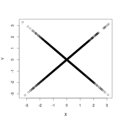
Suppose [math]\displaystyle{ X }[/math] has a normal distribution with expected value 0 and variance 1. Let [math]\displaystyle{ W }[/math] have the Rademacher distribution, so that [math]\displaystyle{ W=1 }[/math] or [math]\displaystyle{ W=-1 }[/math], each with probability 1/2, and assume [math]\displaystyle{ W }[/math] is independent of [math]\displaystyle{ X }[/math]. Let [math]\displaystyle{ Y=WX }[/math]. Then
- [math]\displaystyle{ X }[/math] and [math]\displaystyle{ Y }[/math] are uncorrelated;
- both have the same normal distribution; and
- [math]\displaystyle{ X }[/math] and [math]\displaystyle{ Y }[/math] are not independent.[2]
To see that [math]\displaystyle{ X }[/math] and [math]\displaystyle{ Y }[/math] are uncorrelated, one may consider the covariance [math]\displaystyle{ \operatorname{cov}(X,Y) }[/math]: by definition, it is
- [math]\displaystyle{ \operatorname{cov}(X,Y) = \operatorname E(XY) - \operatorname E(X)\operatorname E(Y). }[/math]
Then by definition of the random variables [math]\displaystyle{ X }[/math], [math]\displaystyle{ Y }[/math], and [math]\displaystyle{ W }[/math], and the independence of [math]\displaystyle{ W }[/math] from [math]\displaystyle{ X }[/math], one has
- [math]\displaystyle{ \operatorname{cov}(X,Y) = \operatorname E(XY) - 0 = \operatorname E(X^2W)=\operatorname E(X^2)\operatorname E(W)=\operatorname E(X^2) \cdot 0=0. }[/math]
To see that [math]\displaystyle{ Y }[/math] has the same normal distribution as [math]\displaystyle{ X }[/math], consider
- [math]\displaystyle{ \begin{align} \Pr(Y \le x) & {} = \operatorname E(\Pr(Y \le x\mid W)) \\ & {} = \Pr(X \le x)\Pr(W = 1) + \Pr(-X\le x)\Pr(W = -1) \\ & {} = \Phi(x) \cdot\frac12 + \Phi(x)\cdot\frac12 \end{align} }[/math]
(since [math]\displaystyle{ X }[/math] and [math]\displaystyle{ -X }[/math] both have the same normal distribution), where [math]\displaystyle{ \Phi(x) }[/math] is the cumulative distribution function of the normal distribution..
To see that [math]\displaystyle{ X }[/math] and [math]\displaystyle{ Y }[/math] are not independent, observe that [math]\displaystyle{ |Y|=|X| }[/math] or that [math]\displaystyle{ \operatorname{Pr}(Y \gt 1 | X = 1/2) = \operatorname{Pr}(X \gt 1 | X = 1/2) = 0 }[/math].
Finally, the distribution of the simple linear combination [math]\displaystyle{ X+Y }[/math] concentrates positive probability at 0: [math]\displaystyle{ \operatorname{Pr}(X+Y=0) = 1/2 }[/math]. Therefore, the random variable [math]\displaystyle{ X+Y }[/math] is not normally distributed, and so also [math]\displaystyle{ X }[/math] and [math]\displaystyle{ Y }[/math] are not jointly normally distributed (by the definition above).
An asymmetric example
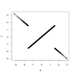
Suppose [math]\displaystyle{ X }[/math] has a normal distribution with expected value 0 and variance 1. Let
- [math]\displaystyle{ Y=\left\{\begin{matrix} X & \text{if } \left|X\right| \leq c \\ -X & \text{if } \left|X\right|\gt c \end{matrix}\right. }[/math]
where [math]\displaystyle{ c }[/math] is a positive number to be specified below. If [math]\displaystyle{ c }[/math] is very small, then the correlation [math]\displaystyle{ \operatorname{corr}(X,Y) }[/math] is near [math]\displaystyle{ -1 }[/math] if [math]\displaystyle{ c }[/math] is very large, then [math]\displaystyle{ \operatorname{corr}(X,Y) }[/math] is near 1. Since the correlation is a continuous function of [math]\displaystyle{ c }[/math], the intermediate value theorem implies there is some particular value of [math]\displaystyle{ c }[/math] that makes the correlation 0. That value is approximately 1.54. In that case, [math]\displaystyle{ X }[/math] and [math]\displaystyle{ Y }[/math] are uncorrelated, but they are clearly not independent, since [math]\displaystyle{ X }[/math] completely determines [math]\displaystyle{ Y }[/math].
To see that [math]\displaystyle{ Y }[/math] is normally distributed—indeed, that its distribution is the same as that of [math]\displaystyle{ X }[/math] —one may compute its cumulative distribution function:
- [math]\displaystyle{ \begin{align}\Pr(Y \leq x) &= \Pr(\{|X| \leq c\text{ and }X \leq x\}\text{ or }\{|X|\gt c\text{ and }-X \leq x\})\\ &= \Pr(|X| \leq c\text{ and }X \leq x) + \Pr(|X|\gt c\text{ and }-X \leq x)\\ &= \Pr(|X| \leq c\text{ and }X \leq x) + \Pr(|X|\gt c\text{ and }X \leq x) \\ &= \Pr(X \leq x), \end{align} }[/math]
where the next-to-last equality follows from the symmetry of the distribution of [math]\displaystyle{ X }[/math] and the symmetry of the condition that [math]\displaystyle{ |X| \leq c }[/math].
In this example, the difference [math]\displaystyle{ X-Y }[/math] is nowhere near being normally distributed, since it has a substantial probability (about 0.88) of it being equal to 0. By contrast, the normal distribution, being a continuous distribution, has no discrete part—that is, it does not concentrate more than zero probability at any single point. Consequently [math]\displaystyle{ X }[/math] and [math]\displaystyle{ Y }[/math] are not jointly normally distributed, even though they are separately normally distributed.[3]
See also
References
- ↑ Hogg, Robert; Tanis, Elliot (2001). "Chapter 5.4 The Bivariate Normal Distribution". Probability and Statistical Inference (6th ed.). pp. 258–259. ISBN 0130272949.
- ↑ UIUC, Lecture 21. The Multivariate Normal Distribution, 21.6:"Individually Gaussian Versus Jointly Gaussian".
- ↑ Edward L. Melnick and Aaron Tenenbein, "Misspecifications of the Normal Distribution", The American Statistician, volume 36, number 4 November 1982, pages 372–373


