Overcompleteness

Overcompleteness is a concept from linear algebra that is widely used in mathematics, computer science, engineering, and statistics (usually in the form of overcomplete frames). It was introduced by R. J. Duffin and A. C. Schaeffer in 1952.

Formally, a subset of the vectors [math]\displaystyle{ \{\phi_i\}_{i\in J} }[/math] of a Banach space [math]\displaystyle{ X }[/math], sometimes called a "system", is complete if every element in [math]\displaystyle{ X }[/math] can be approximated arbitrarily well in norm by finite linear combinations of elements in [math]\displaystyle{ \{\phi_i\}_{i\in J} }[/math]. A system is called overcomplete if it contains more vectors than necessary to be complete, i.e., there exist [math]\displaystyle{ \phi_j \in \{\phi_i\}_{i\in J} }[/math] that can be removed from the system such that [math]\displaystyle{ \{\phi_i\}_{i\in J}\setminus \{\phi_j\} }[/math] remains complete. In research areas such as signal processing and function approximation, overcompleteness can help researchers to achieve a more stable, more robust, or more compact decomposition than using a basis.

Relation between overcompleteness and frames

The theory of frames originates in a paper by Duffin and Schaeffer on non-harmonic Fourier series. A frame is defined to be a set of non-zero vectors [math]\displaystyle{ \{\phi_i\}_{i\in J} }[/math] such that for an arbitrary [math]\displaystyle{ f\in\mathcal{H} }[/math],

[math]\displaystyle{ A\|f\|^2\leq\sum_{i\in J}|\langle f, \phi_i \rangle|^2\leq B\|f\|^2 }[/math]

where [math]\displaystyle{ \langle\cdot,\cdot\rangle }[/math] denotes the inner product, [math]\displaystyle{ A }[/math] and [math]\displaystyle{ B }[/math] are positive constants called bounds of the frame. When [math]\displaystyle{ A }[/math] and [math]\displaystyle{ B }[/math] can be chosen such that [math]\displaystyle{ A=B }[/math], the frame is called a tight frame.

It can be seen that [math]\displaystyle{ \mathcal{H}=\operatorname{span}\{\phi_i\} }[/math]. An example of frame can be given as follows. Let each of [math]\displaystyle{ \{\alpha_i\}_{i=1}^{\infty} }[/math] and [math]\displaystyle{ \{\beta_i\}_{i=1}^{\infty} }[/math] be an orthonormal basis of [math]\displaystyle{ \mathcal{H} }[/math], then

[math]\displaystyle{ \{\phi_i\}_{i=1}^{\infty}=\{\alpha_i\}_{i=1}^{\infty}\cup\{\beta_i\}_{i=1}^{\infty} }[/math]

is a frame of [math]\displaystyle{ \mathcal{H} }[/math] with bounds [math]\displaystyle{ A=B=2 }[/math].

Let [math]\displaystyle{ S }[/math] be the frame operator,

[math]\displaystyle{ Sf=\sum_{i\in J}\langle f, \phi_i \rangle\phi_i }[/math]

A frame that is not a Riesz basis, in which case it consists of a set of functions more than a basis, is said to be overcomplete or redundant. In this case, given [math]\displaystyle{ f\in\mathcal{H} }[/math], it can have different decompositions based on the frame. The frame given in the example above is an overcomplete frame.

When frames are used for function estimation, one may want to compare the performance of different frames. The parsimony of the approximating functions by different frames may be considered as one way to compare their performances.

Given a tolerance [math]\displaystyle{ \epsilon }[/math] and a frame [math]\displaystyle{ F=\{\phi_i\}_{i\in J} }[/math] in [math]\displaystyle{ L^2(\mathbb{R}) }[/math], for any function [math]\displaystyle{ f\in L^2(\mathbb{R}) }[/math], define the set of all approximating functions that satisfy [math]\displaystyle{ \|f-\hat{f}\|\lt \epsilon }[/math]

[math]\displaystyle{ N(f,\epsilon)=\{\hat{f}: \hat{f}=\sum_{i=1}^{k}\beta_i\phi_i, \|f-\hat{f}\|\lt \epsilon\} }[/math]

Then let

[math]\displaystyle{ k_{F}(f,\epsilon)=\inf\{k: \hat{f}\in N(f,\epsilon)\} }[/math]

[math]\displaystyle{ k(f,\epsilon) }[/math] indicates the parsimony of utilizing frame [math]\displaystyle{ F }[/math] to approximate [math]\displaystyle{ f }[/math]. Different [math]\displaystyle{ f }[/math] may have different [math]\displaystyle{ k }[/math] based on the hardness to be approximated with elements in the frame. The worst case to estimate a function in [math]\displaystyle{ L^2(\mathbb{R}) }[/math] is defined as

[math]\displaystyle{ k_F (\epsilon)=\sup_{f\in L^2(\mathbb{R})}\{k_{F}(f,\epsilon)\} }[/math]

For another frame [math]\displaystyle{ G }[/math], if [math]\displaystyle{ k_{F}(\epsilon)\lt k_{G}(\epsilon) }[/math], then frame [math]\displaystyle{ F }[/math] is better than frame [math]\displaystyle{ G }[/math] at level [math]\displaystyle{ \epsilon }[/math]. And if there exists a [math]\displaystyle{ \gamma }[/math] that for each [math]\displaystyle{ \epsilon\lt \gamma }[/math], we have [math]\displaystyle{ k_{F}(\epsilon)\lt k_{G}(\epsilon) }[/math], then [math]\displaystyle{ F }[/math] is better than [math]\displaystyle{ G }[/math] broadly.

Overcomplete frames are usually constructed in three ways.

1. Combine a set of bases, such as wavelet basis and Fourier basis, to obtain an overcomplete frame.
2. Enlarge the range of parameters in some frame, such as in Gabor frame and wavelet frame, to have an overcomplete frame.
3. Add some other functions to an existing complete basis to achieve an overcomplete frame.

An example of an overcomplete frame is shown below. The collected data is in a two-dimensional space, and in this case a basis with two elements should be able to explain all the data. However, when noise is included in the data, a basis may not be able to express the properties of the data. If an overcomplete frame with four elements corresponding to the four axes in the figure is used to express the data, each point would be able to have a good expression by the overcomplete frame.

• 

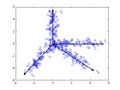  An example of an overcomplete frame

The flexibility of the overcomplete frame is one of its key advantages when used in expressing a signal or approximating a function. However, because of this redundancy, a function can have multiple expressions under an overcomplete frame. When the frame is finite, the decomposition can be expressed as

[math]\displaystyle{ f=Ax }[/math]

where [math]\displaystyle{ f }[/math] is the function one wants to approximate, [math]\displaystyle{ A }[/math] is the matrix containing all the elements in the frame, and [math]\displaystyle{ x }[/math] is the coefficients of [math]\displaystyle{ f }[/math] under the representation of [math]\displaystyle{ A }[/math]. Without any other constraint, the frame will choose to give [math]\displaystyle{ x }[/math] with minimal norm in [math]\displaystyle{ L^2(\mathbb{R}) }[/math]. Based on this, some other properties may also be considered when solving the equation, such as sparsity. So different researchers have been working on solving this equation by adding other constraints in the objective function. For example, a constraint minimizing [math]\displaystyle{ x }[/math]'s norm in [math]\displaystyle{ L^1(\mathbb{R}) }[/math] may be used in solving this equation. This should be equivalent to the Lasso regression in statistics community. Bayesian approach is also used to eliminate the redundancy in an overcomplete frame. Lweicki and Sejnowski proposed an algorithm for overcomplete frame by viewing it as a probabilistic model of the observed data. Recently, the overcomplete Gabor frame has been combined with bayesian variable selection method to achieve both small norm expansion coefficients in [math]\displaystyle{ L^2(\mathbb{R}) }[/math] and sparsity in elements.

Examples of overcomplete frames

In modern analysis in signal processing and other engineering field, various overcomplete frames are proposed and used. Here two common used frames, Gabor frames and wavelet frames, are introduced and discussed.

Gabor frames

In usual Fourier transformation, the function in time domain is transformed to the frequency domain. However, the transformation only shows the frequency property of this function and loses its information in the time domain. If a window function [math]\displaystyle{ g }[/math], which only has nonzero value in a small interval, is multiplied with the original function before operating the Fourier transformation, both the information in time and frequency domains may remain at the chosen interval. When a sequence of translation of [math]\displaystyle{ g }[/math] is used in the transformation, the information of the function in time domain are kept after the transformation.

Let operators

[math]\displaystyle{ T_a: L^2(R)\rightarrow L^2(R), (T_af)(x)=f(x-a) }[/math]

[math]\displaystyle{ E_b: L^2(R)\rightarrow L^2(R), (E_bf)(x)=e^{2\pi ibx}f(x) }[/math]

[math]\displaystyle{ D_c: L^2(R)\rightarrow L^2(R), (D_cf)(x)=\frac{1}{\sqrt c}f\left(\frac{x}{c}\right) }[/math]

A Gabor frame (named after Dennis Gabor and also called Weyl-Heisenberg frame) in [math]\displaystyle{ L^2(R) }[/math] is defined as the form [math]\displaystyle{ \{E_{mb}T_ {na}g\}_{m,n\in Z} }[/math], where [math]\displaystyle{ a,b\gt 0 }[/math] and [math]\displaystyle{ g\in L^2(R) }[/math] is a fixed function. However, not for every [math]\displaystyle{ a }[/math] and [math]\displaystyle{ b }[/math] [math]\displaystyle{ \{E_{mb}T_{na}g\}_{m,n\in Z} }[/math] forms a frame on [math]\displaystyle{ L^2(R) }[/math]. For example, when [math]\displaystyle{ ab\gt 1 }[/math], it is not a frame for [math]\displaystyle{ L^2(R) }[/math]. When [math]\displaystyle{ ab=1 }[/math], [math]\displaystyle{ \{E_{mb}T_{na}g\}_{m,n\in Z} }[/math] is possible to be a frame, in which case it is a Riesz basis. So the possible situation for [math]\displaystyle{ \{E_{mb}T_{na}g\}_{m,n\in Z} }[/math] being an overcomplete frame is [math]\displaystyle{ ab\lt 1 }[/math]. The Gabor family [math]\displaystyle{ \{E_{mb/c}T_{nac}g_c\}_{m,n\in Z} }[/math] is also a frame and sharing the same frame bounds as [math]\displaystyle{ \{E_{mb}T_{na}g\}_{m,n\in Z}. }[/math]

Different kinds of window function [math]\displaystyle{ g }[/math] may be used in Gabor frame. Here examples of three window functions are shown, and the condition for the corresponding Gabor system being a frame is shown as follows.

• 

  Three window functions used in Gabor frame generation.

(1) [math]\displaystyle{ g(x)=e^{-x^2} }[/math], [math]\displaystyle{ \{E_{mb}T_{na}g\}_{m,n\in Z} }[/math] is a frame when [math]\displaystyle{ ab\lt 0.994 }[/math]

(2) [math]\displaystyle{ g(x)=\frac{1}{cosh(\pi x)} }[/math], [math]\displaystyle{ \{E_{mb}T_{na}g\}_{m,n\in Z} }[/math] is a frame when [math]\displaystyle{ ab\lt 1 }[/math]

(3) [math]\displaystyle{ g(x)=I_{[0,c)}(x) }[/math], where [math]\displaystyle{ I(x) }[/math] is the indicator function. The situation for [math]\displaystyle{ \{E_{mb}T_{na}g\}_{m,n\in Z} }[/math] to be a frame stands as follows.

1) [math]\displaystyle{ a\gt c }[/math] or [math]\displaystyle{ a\gt 1 }[/math], not a frame

2) [math]\displaystyle{ c\gt 1 }[/math] and [math]\displaystyle{ a=1 }[/math], not a frame

3) [math]\displaystyle{ a\leq c\leq1 }[/math], is a frame

4) [math]\displaystyle{ a\lt 1 }[/math] and is an irrational, and [math]\displaystyle{ c\in(1,2) }[/math], is a frame

5) [math]\displaystyle{ a=\frac{p}{q}\lt 1 }[/math], [math]\displaystyle{ p }[/math] and [math]\displaystyle{ q }[/math] are relatively primes, [math]\displaystyle{ 2-\frac{1}{q} \lt c\lt 2 }[/math], not a frame

6) [math]\displaystyle{ \frac{3}{4}\lt a\lt 1 }[/math] and [math]\displaystyle{ c=L-1+L(1-a) }[/math], where [math]\displaystyle{ L\geq 3 }[/math] and be a natural number, not a frame

7) [math]\displaystyle{ a\lt 1 }[/math], [math]\displaystyle{ c\gt 1 }[/math], [math]\displaystyle{ |c-[c]-\frac{1}{2}|\lt \frac{1}{2}-a }[/math], where [math]\displaystyle{ [c] }[/math] is the biggest integer not exceeding [math]\displaystyle{ c }[/math], is a frame.

The above discussion is a summary of chapter 8 in.

Wavelet frames

A collection of wavelet usually refers to a set of functions based on [math]\displaystyle{ \psi }[/math]

[math]\displaystyle{ \{2^\frac{j}{2}\psi(2^jx-k)\}_{j,k\in Z} }[/math]

This forms an orthonormal basis for [math]\displaystyle{ L^2(R) }[/math]. However, when [math]\displaystyle{ j,k }[/math] can take values in [math]\displaystyle{ R }[/math], the set represents an overcomplete frame and called undecimated wavelet basis. In general case, a wavelet frame is defined as a frame for [math]\displaystyle{ L^2(R) }[/math] of the form

[math]\displaystyle{ \{a^\frac{j}{2}\psi(a^jx-kb)\}_{j,k\in Z} }[/math]

where [math]\displaystyle{ a\gt 1 }[/math], [math]\displaystyle{ b\gt 0 }[/math], and [math]\displaystyle{ \psi\in L^2(R) }[/math]. The upper and lower bound of this frame can be computed as follows. Let [math]\displaystyle{ \hat{\psi}(\gamma) }[/math] be the Fourier transform for [math]\displaystyle{ \psi\in L^1(R) }[/math]

[math]\displaystyle{ \hat{\psi}(\gamma)=\int_{R}\psi(x)e^{-2\pi ix\gamma}dx }[/math]

When [math]\displaystyle{ a,b }[/math] are fixed, define

[math]\displaystyle{ G_0(\gamma)=\sum_{j\in Z} |\hat{\psi}(a^j\gamma)|^2 }[/math]

[math]\displaystyle{ G_1(\gamma)=\sum_{k\neq0}\sum_{j\in Z} |\hat{\psi}(a^j\gamma)\hat{\psi}(a^j\gamma+\frac{k}{b})| }[/math]

Then

[math]\displaystyle{ B=\frac{1}{b}\sup_{|\gamma|\in[1,a]}(G_0(\gamma)+G_1(\gamma))\lt \infty }[/math]

[math]\displaystyle{ A=\frac{1}{b}\inf_{|\gamma|\in[1,a]}(G_0(\gamma)-G_1(\gamma))\gt 0 }[/math]

Furthermore, when

[math]\displaystyle{ \sum_{j\in Z}|\hat{\psi}(2^j\gamma)|^2=A }[/math]

[math]\displaystyle{ \sum_{j=0}^\infty \hat{\psi}(2^j\gamma)\overline{\hat{\psi}(2^j(\gamma+q))}=0 }[/math], for all odd integers [math]\displaystyle{ q }[/math]

the generated frame [math]\displaystyle{ \{\psi_{j,k}\}_{j,k\in Z} }[/math] is a tight frame.

The discussion in this section is based on chapter 11 in.

Applications

Overcomplete Gabor frames and Wavelet frames have been used in various research area including signal detection, image representation, object recognition, noise reduction, sampling theory, operator theory, harmonic analysis, nonlinear sparse approximation, pseudodifferential operators, wireless communications, geophysics, quantum computing, and filter banks.

References

- ↑ 1.0 1.1 R. J. Duffin and A. C. Schaeffer, A class of nonharmonic Fourier series, Transactions of the American Mathematical Society, vol. 72, no. 2, pp. 341{366, 1952. [Online]. Available: https://www.jstor.org/stable/1990760
- ↑ C. Heil, A Basis Theory Primer: Expanded Edition. Boston, MA: Birkhauser, 2010.
- ↑ 3.0 3.1 R. Balan, P. Casazza, C. Heil, and Z. Landau, Density, overcompleteness, and localization of frames. I. theory, Journal of Fourier Analysis and Applications, vol. 12, no. 2, 2006.
- ↑ K. Grochenig, Foundations of time-frequency analysis. Boston, MA: Birkhauser, 2000.
- ↑ 5.0 5.1 5.2 5.3 5.4 O. Christensen, An Introduction to Frames and Riesz Bases. Boston, MA: Birkhauser, 2003.
- ↑ [1], STA218, Data Mining Class Note at Duke University
- ↑ 7.0 7.1 M. S. Lewicki and T. J. Sejnowski, Learning overcomplete representations, Neural Computation, vol. 12, no. 2, pp. 337{365, 2000.
- ↑ P. Wolfe, S. Godsill, and W. Ng, Bayesian variable selection and regularization for time-frequency surface estimation, J. R. Statist. Soc. B, vol. 66, no. 3, 2004.