Physics:Berman flow
In fluid dynamics, Berman flow is a steady flow created inside a rectangular channel with two equally porous walls, through which fluid is injected from one side and extracted from other side with the constant uniform velocity. The concept is named after a scientist Abraham S. Berman who formulated the problem in 1953.[1]
Flow description
Consider a rectangular channel of width much longer than the height. Let the distance between the top and bottom wall be and choose the coordinates such that lies in the midway between the two walls, with points perpendicular to the planes. Let both walls be porous with equal velocity . Then the continuity equation and Navier–Stokes equations for incompressible fluid become[2]
with boundary conditions
The boundary conditions at the center is due to symmetry. Since the solution is symmetric above the plane , it is enough to describe only half of the flow, say for . If we look for a solution, that is independent of , the continuity equation dictates that the horizontal velocity can at most be a linear function of .[3] Therefore, Berman introduced the following form,
where is the average value (averaged cross-sectionally) of at , that is to say
This constant will be eliminated out of the problem and will have no influence on the solution. Substituting this into the momentum equation leads to
Differentiating the second equation with respect to gives this can substituted into the first equation after taking the derivative with respect to which leads to
where is the Reynolds number. Integrating once, we get
with boundary conditions
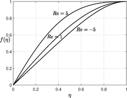
This third order nonlinear ordinary differential equation requires three boundary condition and the fourth boundary condition is to determine the constant . and this equation is found to possess multiple solutions.[4][5] The figure shows the numerical solution for low Reynolds number, solving the equation for large Reynolds number is not a trivial computation.
Limiting solutions
In the limit , the solution can be written as
In the limit , the leading-order solution is given by[6]
The above solution satisfies all the necessary boundary conditions even though Reynolds number is infinite (see also Taylor–Culick flow)
Axisymmetric case
The corresponding problem in porous pipe flows was addressed by S. W. Yuan and A. Finkelstein in 1955.[7]
See also
References
- ↑ Berman, Abraham S. "Laminar flow in channels with porous walls." Journal of Applied physics 24.9 (1953): 1232–1235.
- ↑ Drazin, P. G., & Riley, N. (2006). The Navier-Stokes equations: a classification of flows and exact solutions (No. 334). Cambridge University Press.
- ↑ Proudman, I. (1960). An example of steady laminar flow at large Reynolds number. Journal of Fluid Mechanics, 9(4), 593-602.
- ↑ Wang, C-A., T-W. Hwang, and Y-Y. Chen. "Existence of solutions for Berman's equation from Laminar flows in a porous channel with suction." Computers & Mathematics with Applications 20.2 (1990): 35–40.
- ↑ Hwang, Tzy-Wei, and Ching-An Wang. "On multiple solutions for Berman's problem." Proceedings of the Royal Society of Edinburgh: Section A Mathematics 121.3-4 (1992): 219–230.
- ↑ Morduchow, M. (1957). On laminar flow through a channel or tube with injection: application of method of averages. Quarterly of Applied Mathematics, 14(4), 361-368.
- ↑ Yuan, S. W., Finkelstein, A. (1955). Laminar pipe flow with injection and suction through a porous wall. PRINCETON UNIV NJ JAMES FORRESTAL RESEARCH CENTER.
 |  |

