Physics:Dimensionless momentum-depth relationship in open-channel flow
Momentum in open channel flow
Momentum for one-dimensional flow
Momentum for one-dimensional flow in a channel can be given by the expression: [math]\displaystyle{ M=\frac{Q^2}{gA}+\overline yA }[/math] where:
- M is the momentum [L3]
- Q is the rate of flow [L3/s]
- g is the acceleration due to gravity [L/T2]
- A is the cross sectional area of flow [L2]
- ȳ is the distance from the centroid of A to the water surface [L]
For open channel flow calculations where momentum can be assumed to be conserved, such as in a hydraulic jump, we[who?] can equate the Momentum at an upstream location, M1, to that at a downstream location, M2, such that: [math]\displaystyle{ M_1=\frac{Q^2}{gA_1}+\overline y_1A_1=\frac{Q^2}{gA_2}+\overline y_2A_2=M_2 }[/math]
Momentum in a rectangular channel
In the unique circumstance where the flow is in a rectangular channel (such as a laboratory flume), we can describe this relationship as unit momentum, by dividing both sides of the equation by the width of the channel. This produces uM in terms of ft2, and is given by the equation: [math]\displaystyle{ {_uM_1}=\frac{q^2}{gy_1}+ \frac{y_1^2}{2} =\frac{q^2}{gy_2}+ \frac{y_2^2}{2}={_uM_2} }[/math] where:
- uM is M/b [L2]
- q is Q/b [L2/T]
- b is the base width of the rectangular channel [L]
Importance of momentum in open channel flow
Momentum is one of the most important basic definitions in Fluid Mechanics. The conservation of momentum is one of the three fundamental physical principles in both Fluid Mechanics and [Open-channel flow | open channel flow] (the other two are mass conservation and energy conservation). This principle leads to the momentum equation set in three dimensions (x, y and z). With different assumptions, these momentum equations can be simplified to several widely applied forms:
With Newton’s second law, Newtonian fluids assumption and Stokes hypothesis, the original fluid momentum equations are derived as the Navier–Stokes equations. These equations are classic in Fluid Mechanics, but the nonlinearity in these partial differential equations make them difficult to solve mathematically. As a result, analytical solutions for the Navier–Stokes equations still remain a tough research topic.
For high Reynolds number flow, the effects of viscosity are negligible. In these cases, with the inviscid assumption, Navier–Stokes equations can be derived as Euler equations. Though they are still nonlinear partial differential equations, the elimination of viscous terms simplifies the problem.
In some applications, when viscosity, rotationality and compressibility of the fluid can be neglected, the Navier–Stokes equations can be further simplified to the Laplace equation form, which is referred as potential flow.
In computational fluid dynamics, solving the partial differential momentum equations mentioned above with discretized algebraic equations is the most important procedure to study flow characteristics in different applications.
Momentum also allows us to describe the characteristics of flow when energy is not conserved. HEC-RAS, a widely used computer model developed by the US Army Corps of Engineers for calculating water surface profiles, considers that when flow passes through critical depth, the basic assumption of gradually varied flow required for the energy equation is not applicable. Locations where flow may make such a transition include: significant changes in slope, channel geometry (e.g. bridge sections), grade control structures, and the confluence of water bodies. In these instances, HEC-RAS will use a form of the momentum equation to solve for the water surface elevation at an unknown location.
In addition, momentum flux is one of the parameters to estimate fluid impact on offshore structures. Analysis of momentum flux in coastal regions can provide advisable infrastructure layout planning to minimize the potential hazards from extreme events such as storm surge, hurricane and tsunami (e.g. (Park et al. 2013), (Yeh 2006), (Guard et al. 2005) and (Chanson et al. 2002)).
Characteristics
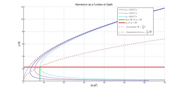
For discussion, we will consider an ideal, frictionless, rectangular channel. For each value of q, a unique curve can be produced where M is shown as a function of depth. As is the case for specific energy, the minimum value of uM, uMmin, corresponds to critical depth. For each value of uM greater than uMmin, there are two depths that can occur. These are called conjugate depths, and represent supercritical and subcritical alternatives for flow of a given uM. Since hydraulic jumps conserve momentum, if the depth at the upstream or downstream end of a hydraulic jump is known, we can determine the unknown depth by drawing a vertical line through the known depth and reading its conjugate. The M-y diagram below shows three M-y curves with unit discharge 10, 15 and 1.85806 m2/s. It can be observed that the M-y curves shift in positive M axis as the q value increases. From the M-y equation mentioned earlier, as y increases to infinity, the q2 / gy1 term would be negligible, and the M value will converge to 0.5y2 (shown as the black dashed curve in M-y diagram). By taking the derivative dM / dy = 0, we can also obtain the equation of minimum M with different q values: [math]\displaystyle{ \frac{dM}{dy} = y_c - \frac{q^2}{gy_c^2} }[/math]
By eliminating the term of q in the equation above with the relationship between q and yc (yc = ( q2 / g )1/3 ), and put the resulting equation of y into the original M-y ccg3 c equation, we can obtain the characteristic curve of critical M and y (shown as the red dashed curve in M-y diagram): [math]\displaystyle{ y_c = \frac{2}{3}\sqrt{M_c} }[/math]
Dimensionless M’-y’ diagram
Motivation for dimensionless momentum–depth relationship
Conjugate depths can be determined from curves like the one above. However, since this curve is unique for q = 1.85806 m2/s, we would have to develop a new curve for each rectangular channel of a given base width (or discharge). If we can establish a dimensionless relationship, we can apply the curve to any problem in which the cross-section is rectangular in shape. To create a dimensionless momentum–depth relationship, we will divide both sides by a normalizing value that will allow us to use a dimensionless relationship between Momentum and Depth for all values of q.
Derivation of the dimensionless momentum–depth relationship
Given that: [math]\displaystyle{ {_uM_1}=\frac{q^2}{gy_1}+ \frac{y_1^2}{2} =\frac{q^2}{gy_2}+ \frac{y_2^2}{2}={_uM_2} }[/math] and that: [math]\displaystyle{ {q^2}={gy_c^3} }[/math] according to the Buckingham π theorem, with dimensional analysis, we can normalize the relationship between depth and Momentum by dividing both by the value of the critical depth squared and substituting for q2 to yield: [math]\displaystyle{ \frac{_uM}{y_c^2} = \frac{gy_c^3}{gyy_c^2} + \frac{y^2}{2y_c^2} }[/math] where yc is the critical depth.
If we let M’ = uM/yc2, and y’ = y/yc, this equation becomes: [math]\displaystyle{ M'= \frac{1}{y'} + \frac{y'^2}{2} }[/math]
The dimensionless momentum–depth diagram
By applying the conversion to dimensionless units described above, the dimensionless momentum–depth diagram is produced below.

Relationship to the dimensionless energy–depth diagram
By close inspection of the dimensionless dnergy–depth diagram, an interesting conclusion can be drawn, which is that M’ is the same function of y’ as E’ is of 1/y’, and vice versa. This is demonstrated in the following chart that compares favorably to the chart of the Dimensionless Energy-Depth Diagram. Note that the only difference between the chart above and the one below is the values of the y-axis are the reciprocal of one another and that the scale has been changed to be consistent with the scale found in the discussion of Dimensionless Energy-Depth.

Because Energy and Momentum have this reciprocal relationship (found also in the non-dimensionless forms of these relationships), we can use a Dimensionless Energy-Depth Diagram to create a dimensionless momentum–depth diagram, and vice versa.
Solution of simple version of hydraulic jump with dimensionless diagram
To demonstrate the use of a dimensionless momentum–depth diagram in the solution of a simple hydraulic jump problem (hydraulic jump is also very common in other situations. Let’s consider a rectangular channel with a base width of 3.048 m, and a flow rate of 2.831 m3/s, with a tailwater induced downstream depth of 1.828 m. What is the depth of flow at the upstream end of the hydraulic jump?
Step 1 – Calculate q: [math]\displaystyle{ q = \frac{Q}{b} = \frac{100 \mathrm{ft^3/s}}{10 \mathrm{ft}}=10ft^2/s }[/math]
Step 2 – Calculate yc: [math]\displaystyle{ y_c=\sqrt[3]{q^2 \over g} = \sqrt[3]{{(10 \mathrm{ft^2/s})}^2 \over 32.2 \mathrm{ft/s^2}}=1.459 \mathrm{ft} }[/math] (note-calculations are displayed to 3 decimal places to reduce rounding errors in Step 6)
Step 3 – Calculate y′ for the downstream depth: [math]\displaystyle{ y'=\frac{y_d}{y_c} = \frac{6 \mathrm{ft}}{1.46 \mathrm{ft}} = 4.112 }[/math]
Step 4 – Determine Conjugate Dimensionless Depth from Chart:
Using the Dimensionless Chart presented above, plot y′ = 4.11 over to its intersection with the M’ curve. Read down the chart to find the conjugate depth and determine the new y′ from the left axis.

Step 5 – Calculate the upstream (conjugate) depth to 1.828 m by converting y′ = 0.115 to its actual depth: [math]\displaystyle{ y'=\frac{y_u}{y_c} \implies {y_u}={y'}{y_c}=0.115(1.459\mathrm{ft})=0.168 \mathrm{ft} }[/math] Step 6 – Validation: [math]\displaystyle{ {_uM_u}=\frac{q^2}{gy_1}+ \frac{y_1^2}{2} = \frac{10^2}{(32.2)0.168}+ \frac{0.168^2}{2} = 18.500\mathrm{ft^2} }[/math] and [math]\displaystyle{ {_uM_d}=\frac{q^2}{gy_2}+ \frac{y_2^2}{2} = \frac{10^2}{(32.2)6} + \frac{6^2}{2} = 18.518\mathrm{ft^2} }[/math]
The difference between uMu and uMd is shown as 0.001553575731 m2 due to rounding errors. Therefore, uMu and uMd are shown to represent the same unit momentum across the jump and momentum is conserved, validating the calculations using the Dimensionless Chart above.
This topic contribution was made in partial fulfillment of the requirements for Virginia Tech, Department of Civil and Environmental Engineering course: CEE 5984 – Open Channel Flow during the Fall 2010 semester.
Solution of hydraulic jump with sluice gate
The following example of a hydraulic jump at a sluice gate outlet will give a clear idea about how conservation of energy and conservation of momentum apply in open channel flow.
As shown in the middle panel in schematic plot, in a rectangular channel, deep upstream flow (position 1) encounters a sluice gate in front of position 2. A sluice gate imposes adecrease in flow depth at position 2, and a hydraulic jump is formed between position 2 and far downstream where the flow depth increases again (position 3). The left panel in Figure 2 shows the M-y diagram of these 3 positions (momentum is also referred to as other definitions in different references, e.g. “Specific Force” in (Chaudhry 2008)), while the right panel in schematic plot shows the E-y diagram for these 3 positions. Energy loss can be neglected between position 1 and 2 (e.g. assuming conservation of energy), but the external thrust on the gate causes significant momentum loss. By contrast, between positions 2 and 3, turbulence in the hydraulic jump dissipates energy, while the momentum can be assumed to be conserved. If we know the unit discharge as q = 0.929 m2/s and the flow depth at position 1 as y1 = 2.438 m, by applying energy conservation between position 1 & 2 and momentum conservation between 2 & 3, the flow depths at position 2 (y2) and 3 (y3) can be computed.
Applying conservation of energy between position 1 & 2: [math]\displaystyle{ E_1 = E_2 }[/math] [math]\displaystyle{ y_1 + \frac{q^2}{2gy_1} = y_2 + \frac{q^2}{2gy_2} = 8.02 \mathrm{ft} }[/math] [math]\displaystyle{ y_2 = \frac{2y_1}{-1 + \sqrt{1+8\frac{gy_1^3}{q^2}}} =0.45 \mathrm{ft} }[/math]
Applying conservation of momentum between position 2 & 3: [math]\displaystyle{ M_2 = M_3 }[/math] [math]\displaystyle{ \frac{y_2}{2} + \frac{q^2}{gy_2} = \frac{y_3}{2} + \frac{q^2}{gy_3} = 32.4 \mathrm{ft} }[/math] [math]\displaystyle{ y_3 = \frac{y_2}{2} \left(-1 + \sqrt{1+8\frac{q^2}{gy_2^3}}\right) = 3.46 \mathrm{ft} }[/math]
In addition, we can obtain the thrust on the sluice gate as well: [math]\displaystyle{ \triangle M = M_1 - M_2 = 25.5 }[/math] [math]\displaystyle{ \text{Thrust} = \gamma \triangle M = \rho g \triangle M = 1590 \mathrm{lbs/ff} }[/math]
(The example above comes from Dr. Moglen’s “Open Channel Flow” course (CEE5384) in Virginia Tech, U.S.)

References
- Brunner, G.W., HEC-RAS, River Analysis System Hydraulic Reference Manual (CPD-69), US Army Corps of Engineers, Hydrologic Engineering Center, 2010.
- Chanson, H., Aoki, S.-i. & Maruyama, M. (2002), ‘An experimental study of tsunami runup on dry and wet horizontal coastlines’, Science of Tsunami Hazards 20(5), 278–293.
- Chaudhry, M.H., Open-Channel Flow (second edition), Springer Science+Business Media, llc, 2008.
- French, R.H., Open-Channel Hydraulics, McGraw-Hill, Inc., 1985.
- Guard, P., Baldock, T. & Nielsen, P. (2005), General solutions for the initial run-up of a breaking tsunami front, in ‘International Symposium Disaster Reduction on Coasts’, Monash University, pp. 1–8.
- Henderson, F.M., Open Channel Flow, Prentice-Hall, 1966.
- Janna, W.S., Introduction to Fluid Mechanics, PWS-Kent Publishing Company, 1993.
- Linsey, R.K., Franzini, J.B., Freyberg, D.L., Tchobanoglous, G., Water-Resources Engineering (fourth edition), McGraw-Hill, Inc., 1992.
- Park, H., Cox, D. T., Lynett, P. J., Wiebe, D. M. & Shin, S. (2013), ‘Tsunami inunda- tion modeling in constructed environments: A physical and numerical comparison of free-surface elevation, velocity, and momentum flux’, Coastal Engineering 79, 9– 21.
- Yeh, H. (2006), ‘Maximum fluid forces in the tsunami runup zone’, Journal of water- way, port, coastal, and ocean engineering 132(6), 496–500.
 |

