Physics:Landau theory

Short description: Theory of continuous phase transitions

Landau theory (also known as Ginzburg–Landau theory, despite the confusing name) in physics is a theory that Lev Landau introduced in an attempt to formulate a general theory of continuous (i.e., second-order) phase transitions. It can also be adapted to systems under externally-applied fields, and used as a quantitative model for discontinuous (i.e., first-order) transitions. Although the theory has now been superseded by the renormalization group and scaling theory formulations, it remains an exceptionally broad and powerful framework for phase transitions, and the associated concept of the order parameter as a descriptor of the essential character of the transition has proven transformative.

Mean-field formulation (no long-range correlation)

Landau was motivated to suggest that the free energy of any system should obey two conditions:

• Be analytic in the order parameter and its gradients.
• Obey the symmetry of the Hamiltonian.

Given these two conditions, one can write down (in the vicinity of the critical temperature, T_c) a phenomenological expression for the free energy as a Taylor expansion in the order parameter.

Second-order transitions

Sketch of free energy as a function of order parameter [math]\displaystyle{ \eta }[/math]

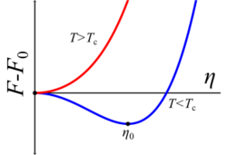
Consider a system that breaks some symmetry below a phase transition, which is characterized by an order parameter [math]\displaystyle{ \eta }[/math]. This order parameter is a measure of the order before and after a phase transition; the order parameter is often zero above some critical temperature and non-zero below the critical temperature. In a simple ferromagnetic system like the Ising model, the order parameter is characterized by the net magnetization [math]\displaystyle{ m }[/math], which becomes spontaneously non-zero below a critical temperature [math]\displaystyle{ T_c }[/math]. In Landau theory, one considers a free energy functional that is an analytic function of the order parameter. In many systems with certain symmetries, the free energy will only be a function of even powers of the order parameter, for which it can be expressed as the series expansion

[math]\displaystyle{ F(T,\eta) - F_0 = a(T) \eta^2 + \frac{b(T)}{2} \eta^4 + \cdots }[/math]

In general, there are higher order terms present in the free energy, but it is a reasonable approximation to consider the series to fourth order in the order parameter, as long as the order parameter is small. For the system to be thermodynamically stable (that is, the system does not seek an infinite order parameter to minimize the energy), the coefficient of the highest even power of the order parameter must be positive, so [math]\displaystyle{ b(T)\gt 0 }[/math]. For simplicity, one can assume that [math]\displaystyle{ b(T) = b_0 }[/math], a constant, near the critical temperature. Furthermore, since [math]\displaystyle{ a(T) }[/math] changes sign above and below the critical temperature, one can likewise expand [math]\displaystyle{ a(T) \approx a_0 (T-T_c) }[/math], where it is assumed that [math]\displaystyle{ a\gt 0 }[/math] for the high-temperature phase while [math]\displaystyle{ a\lt 0 }[/math] for the low-temperature phase, for a transition to occur. With these assumptions, minimizing the free energy with respect to the order parameter requires

[math]\displaystyle{ \frac{\partial F}{\partial \eta} = 2a(T) \eta + 2b(T) \eta^3 = 0 }[/math]

The solution to the order parameter that satisfies this condition is either [math]\displaystyle{ \eta= 0 }[/math], or

[math]\displaystyle{ \eta_0^2 = -\frac{a}{b} = - \frac{a_0}{b_0}(T-T_c) }[/math]

Order parameter and specific heat as a function of temperature

It is clear that this solution only exists for [math]\displaystyle{ T\lt T_c }[/math], otherwise [math]\displaystyle{ \eta= 0 }[/math] is the only solution. Indeed, [math]\displaystyle{ \eta= 0 }[/math] is the minimum solution for [math]\displaystyle{ T\gt T_c }[/math], but the solution [math]\displaystyle{ \eta_0 }[/math] minimizes the free energy for [math]\displaystyle{ T\lt T_c }[/math], and thus is a stable phase. Furthermore, the order parameter follows the relation

[math]\displaystyle{ \eta(T) \propto \left| T - T_c \right|^{1/2} }[/math]

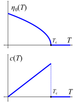
below the critical temperature, indicating a critical exponent [math]\displaystyle{ \beta = 1/2 }[/math] for this Landau mean-theory model.

The free-energy will vary as a function of temperature given by

[math]\displaystyle{ F - F_0 = \begin{cases} - \dfrac{a_0^2}{2b_0} (T-T_c)^2, & T\lt T_c \\ 0, & T\gt T_c \end{cases} }[/math]

From the free energy, one can compute the specific heat,

[math]\displaystyle{ c_p = -T\frac{\partial^2 F}{\partial T^2} = \begin{cases} \dfrac{a_0^2}{b_0} T, & T\lt T_c \\ 0, & T\gt T_c \end{cases} }[/math]

which has a finite jump at the critical temperature of size [math]\displaystyle{ \Delta c = a_0^2 T_c/b_0 }[/math]. This finite jump is therefore not associated with a discontinuity that would occur if the system absorbed latent heat, since [math]\displaystyle{ T_c \Delta S = 0 }[/math]. It is also noteworthy that the discontinuity in the specific heat is related to the discontinuity in the second derivative of the free energy, which is characteristic of a second-order phase transition. Furthermore, the fact that the specific heat has no divergence or cusp at the critical point indicates its critical exponent for [math]\displaystyle{ c\sim |T-T_c|^{-\alpha} }[/math] is [math]\displaystyle{ \alpha=0 }[/math].

Applied fields

In many systems, one can consider a perturbing field [math]\displaystyle{ h }[/math] that couples linearly to the order parameter. For example, in the case of a classical dipole moment [math]\displaystyle{ \mu }[/math], the energy of the dipole-field system is [math]\displaystyle{ -\mu B }[/math]. In the general case, one can assume an energy shift of [math]\displaystyle{ -\eta h }[/math] due to the coupling of the order parameter to the applied field [math]\displaystyle{ h }[/math], and the Landau free energy will change as a result:

[math]\displaystyle{ F(T,\eta) - F_0 = a_0 (T-T_c) \eta^2 + \frac{b_0}{2} \eta^4 - \eta h }[/math]

In this case, the minimization condition is

[math]\displaystyle{ \frac{\partial F}{\partial \eta} = 2 a(T) \eta + 2b_0 \eta^3 - h = 0 }[/math]

One immediate consequence of this equation and its solution is that, if the applied field is non-zero, then the magnetization is non-zero at any temperature. This implies there is no longer a spontaneous symmetry breaking that occurs at any temperature. Furthermore, some interesting thermodynamic and universal quantities can be obtained from this above condition. For example, at the critical temperature where [math]\displaystyle{ a(T_c)=0 }[/math], one can find the dependence of the order parameter on the external field:

[math]\displaystyle{ \eta(T_c) = \left( \frac{h}{2b_0} \right)^{1/3} \propto h^{1/\delta} }[/math]

indicating a critical exponent [math]\displaystyle{ \delta = 3 }[/math].

Zero-field susceptibility as a function of temperature near the critical temperature

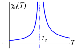
Furthermore, from the above condition, it is possible to find the zero-field susceptibility [math]\displaystyle{ \chi\equiv \partial \eta/\partial h|_{h=0} }[/math], which must satisfy

[math]\displaystyle{ 0 = 2 a \frac{\partial \eta}{\partial h} + 6b \eta^2 \frac{\partial \eta}{\partial h} - 1 }[/math]

[math]\displaystyle{ [2 a + 6b \eta^2] \frac{\partial \eta}{\partial h} = 1 }[/math]

In this case, recalling in the zero-field case that [math]\displaystyle{ \eta^2 = -a/b }[/math] at low temperatures, while [math]\displaystyle{ \eta^2=0 }[/math] for temperatures above the critical temperature, the zero-field susceptibility therefore has the following temperature dependence:

[math]\displaystyle{ \chi(T,h\to 0) = \begin{cases} \frac{1}{2a_0(T-T_c)}, & T\gt T_c \\ \frac{1}{-4a_0(T-T_c)}, & T\lt T_c \end{cases} \propto |T-T_c|^{-\gamma} }[/math]

which is reminiscent of the Curie-Weiss law for the temperature dependence of magnetic susceptibility in magnetic materials, and yields the mean-field critical exponent [math]\displaystyle{ \gamma=1 }[/math].

It is noteworthy that although the critical exponents so obtained are incorrect for many models and systems, they correctly satisfy various exponent equalities such as the Rushbrook equality: [math]\displaystyle{ \alpha + 2\beta + \gamma = 1 }[/math].

First-order transitions

Landau theory can also be used to study first-order transitions. There are two different formulations, depending on whether or not the system is symmetric under a change in sign of the order parameter.

I. Symmetric Case

Here we consider the case where the system has a symmetry and the energy is invariant when the order parameter changes sign. A first-order transition will arise if the quartic term in [math]\displaystyle{ F }[/math] is negative. To ensure that the free energy remains positive at large [math]\displaystyle{ \eta }[/math], one must carry the free-energy expansion to sixth-order,

[math]\displaystyle{ F(T,\eta) = A(T) \eta^2 - B_0 \eta^4 + C_0 \eta^6, }[/math]

where [math]\displaystyle{ A(T)=A_0(T-T_0) }[/math], and [math]\displaystyle{ T_0 }[/math] is some temperature at which [math]\displaystyle{ A(T) }[/math] changes sign. We denote this temperature by [math]\displaystyle{ T_0 }[/math] and not [math]\displaystyle{ T_c }[/math], since it will emerge below that it is not the temperature of the first-order transition, and since there is no critical point, the notion of a "critical temperature" is misleading to begin with. [math]\displaystyle{ A_0, B_0, }[/math] and [math]\displaystyle{ C_0 }[/math] are positive coefficients.

We analyze this free energy functional as follows: (i) For [math]\displaystyle{ T \gt T_0 }[/math], the [math]\displaystyle{ \eta^2 }[/math] and [math]\displaystyle{ \eta^6 }[/math] terms are concave upward for all [math]\displaystyle{ \eta }[/math], while the [math]\displaystyle{ \eta^4 }[/math] term is concave downward. Thus for sufficiently high temperatures [math]\displaystyle{ F }[/math] is concave upward for all [math]\displaystyle{ \eta }[/math], and the equilibrium solution is [math]\displaystyle{ \eta = 0 }[/math]. (ii) For [math]\displaystyle{ T \lt T_0 }[/math], both the [math]\displaystyle{ \eta^2 }[/math] and [math]\displaystyle{ \eta^4 }[/math] terms are negative, so [math]\displaystyle{ \eta = 0 }[/math] is a local maximum, and the minimum of [math]\displaystyle{ F }[/math] is at some non-zero value [math]\displaystyle{ \pm\eta_0(T) }[/math], with [math]\displaystyle{ F(T_0,\eta_0(T_0)) \lt 0 }[/math]. (iii) For [math]\displaystyle{ T }[/math] just above [math]\displaystyle{ T_0 }[/math], [math]\displaystyle{ \eta = 0 }[/math] turns into a local minimum, but the minimum at [math]\displaystyle{ \eta_0(T) }[/math] continues to be the global minimum since it has a lower free energy. It follows that as the temperature is raised above [math]\displaystyle{ T_0 }[/math], the global minimum cannot continuously evolve from [math]\displaystyle{ \eta_0(T) }[/math] to 0. Rather, at some intermediate temperature [math]\displaystyle{ T_* }[/math], the minima at [math]\displaystyle{ \eta_0(T_*) }[/math] and [math]\displaystyle{ \eta = 0 }[/math] must become degenerate. For [math]\displaystyle{ T \gt T_* }[/math], the global minimum will jump discontinuously from [math]\displaystyle{ \eta_0(T_*) }[/math] to 0.

To find [math]\displaystyle{ T_* }[/math], we demand that free energy be zero at [math]\displaystyle{ \eta = \eta_0(T_*) }[/math] (just like the [math]\displaystyle{ \eta=0 }[/math] solution), and furthermore that this point should be a local minimum. These two conditions yield two equations,

[math]\displaystyle{ 0=A(T) \eta^2 - B_0 \eta^4 + C_0 \eta^6, }[/math]

[math]\displaystyle{ 0=2A(T) \eta - 4 B_0 \eta^3 + 6 C_0 \eta^5, }[/math]

First-order phase transition demonstrated in the discontinuity of the order parameter as a function of temperature

which are satisfied when [math]\displaystyle{ \eta^2(T_*) = {B_0}/{2C_0} }[/math]. The same equations also imply that [math]\displaystyle{ A(T_*) = A_0(T_*-T_0) = B_0^2/4C_0 }[/math]. That is,

[math]\displaystyle{ T_* = T_0 + \frac{B_0^2}{4 A_0 C_0}. }[/math]

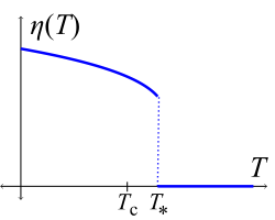
From this analysis both points made above can be seen explicitly. First, the order parameter suffers a discontinuous jump from [math]\displaystyle{ (B_0/2C_0)^{1/2} }[/math] to 0. Second, the transition temperature [math]\displaystyle{ T_* }[/math] is not the same as the temperature [math]\displaystyle{ T_0 }[/math] where [math]\displaystyle{ A(T) }[/math] vanishes.

At temperatures below the transition temperature, [math]\displaystyle{ T\lt T_* }[/math], the order parameter is given by

[math]\displaystyle{ \eta_0^2 = \frac{B_0}{3C_0} \left[ 1 + \sqrt{1 - \frac{3A(T) C_0}{B_0^2}} \right] }[/math]

which is plotted to the right. This shows the clear discontinuity associated with the order parameter as a function of the temperature. To further demonstrate that the transition is first-order, one can show that the free energy for this order parameter is continuous at the transition temperature [math]\displaystyle{ T_* }[/math], but its first derivative (the entropy) suffers from a discontinuity, reflecting the existence of a non-zero latent heat.

II. Nonsymmetric Case

Next we consider the case where the system does not have a symmetry. In this case there is no reason to keep only even powers of [math]\displaystyle{ \eta }[/math] in the expansion of [math]\displaystyle{ F }[/math], and a cubic term must be allowed (The linear term can always be eliminated by a shift [math]\displaystyle{ \eta \to \eta }[/math] + constant.) We thus consider a free energy functional

[math]\displaystyle{ F(T,\eta) = A(T) \eta^2 - C_0 \eta^3 + B_0 \eta^4 + \cdots. }[/math]

Once again [math]\displaystyle{ A(T)=A_0(T-T_0) }[/math], and [math]\displaystyle{ A_0, B_0, C_0 }[/math] are all positive. The sign of the cubic term can always be chosen to be negative as we have done by reversing the sign of [math]\displaystyle{ \eta }[/math] if necessary.

We analyze this free energy functional as follows: (i) For [math]\displaystyle{ T \lt T_0 }[/math], we have a local maximum at [math]\displaystyle{ \eta = 0 }[/math], and since the free energy is bounded below, there must be two local minima at nonzero values [math]\displaystyle{ \eta_-(T) \lt 0 }[/math] and [math]\displaystyle{ \eta_+(T) \gt 0 }[/math]. The cubic term ensures that [math]\displaystyle{ \eta_+ }[/math] is the global minimum since it is deeper. (ii) For [math]\displaystyle{ T }[/math] just above [math]\displaystyle{ T_0 }[/math], the minimum at [math]\displaystyle{ \eta_- }[/math] disappears, the maximum at [math]\displaystyle{ \eta = 0 }[/math] turns into a local minimum, but the minimum at [math]\displaystyle{ \eta_+ }[/math] persists and continues to be the global minimum. As the temperature is further raised, [math]\displaystyle{ F(T,\eta_+(T)) }[/math] rises until it equals zero at some temperature [math]\displaystyle{ T_* }[/math]. At [math]\displaystyle{ T_* }[/math] we get a discontinuous jump in the global minimum from [math]\displaystyle{ \eta_+(T_*) }[/math] to 0. (The minima cannot coalesce for that would require the first three derivatives of [math]\displaystyle{ F }[/math] to vanish at [math]\displaystyle{ \eta = 0 }[/math].)

To find [math]\displaystyle{ T_* }[/math], we demand that free energy be zero at [math]\displaystyle{ \eta = \eta_+(T_*) }[/math] (just like the [math]\displaystyle{ \eta=0 }[/math] solution), and furthermore that this point should be a local minimum. These two conditions yield two equations,

[math]\displaystyle{ 0=A(T) \eta^2 - C_0 \eta^3 + B_0 \eta^4, }[/math]

[math]\displaystyle{ 0=2A(T) \eta - 3 C_0 \eta^2 + 4 B_0 \eta^3, }[/math]

which are satisfied when [math]\displaystyle{ \eta(T_*) = {C_0}/{2B_0} }[/math]. The same equations also imply that [math]\displaystyle{ A(T_*) = A_0(T_*-T_0) = C_0^2/4B_0 }[/math]. That is,

[math]\displaystyle{ T_* = T_0 + \frac{C_0^2}{4 A_0 B_0}. }[/math]

As in the symmetric case the order parameter suffers a discontinuous jump from [math]\displaystyle{ (C_0/2B_0) }[/math] to 0. Second, the transition temperature [math]\displaystyle{ T_* }[/math] is not the same as the temperature [math]\displaystyle{ T_0 }[/math] where [math]\displaystyle{ A(T) }[/math] vanishes.

Applications

It was known experimentally that the liquid–gas coexistence curve and the ferromagnet magnetization curve both exhibited a scaling relation of the form [math]\displaystyle{ |T - T_c|^{\beta} }[/math], where [math]\displaystyle{ \beta }[/math] was mysteriously the same for both systems. This is the phenomenon of universality. It was also known that simple liquid–gas models are exactly mappable to simple magnetic models, which implied that the two systems possess the same symmetries. It then followed from Landau theory why these two apparently disparate systems should have the same critical exponents, despite having different microscopic parameters. It is now known that the phenomenon of universality arises for other reasons (see Renormalization group). In fact, Landau theory predicts the incorrect critical exponents for the Ising and liquid–gas systems.

The great virtue of Landau theory is that it makes specific predictions for what kind of non-analytic behavior one should see when the underlying free energy is analytic. Then, all the non-analyticity at the critical point, the critical exponents, are because the equilibrium value of the order parameter changes non-analytically, as a square root, whenever the free energy loses its unique minimum.

The extension of Landau theory to include fluctuations in the order parameter shows that Landau theory is only strictly valid near the critical points of ordinary systems with spatial dimensions higher than 4. This is the upper critical dimension, and it can be much higher than four in more finely tuned phase transition. In Mukhamel's analysis of the isotropic Lifschitz point, the critical dimension is 8. This is because Landau theory is a mean field theory, and does not include long-range correlations.

This theory does not explain non-analyticity at the critical point, but when applied to superfluid and superconductor phase transition, Landau's theory provided inspiration for another theory, the Ginzburg–Landau theory of superconductivity.

Including long-range correlations

Consider the Ising model free energy above. Assume that the order parameter [math]\displaystyle{ \Psi }[/math] and external magnetic field, [math]\displaystyle{ h }[/math], may have spatial variations. Now, the free energy of the system can be assumed to take the following modified form:

[math]\displaystyle{ F := \int d^D x \ \left( a(T) + r(T) \psi^2(x) + s(T) \psi^4(x) \ + f(T) (\nabla \psi(x))^2 \ +h(x) \psi(x)\ \ + \mathcal{O}(\psi^6 ; (\nabla \psi)^4) \right) }[/math]

where [math]\displaystyle{ D }[/math] is the total spatial dimensionality. So,

[math]\displaystyle{ \langle \psi(x) \rangle := \frac{\text{Tr}\ \psi(x) {\rm e}^{-\beta H}}{Z} }[/math]

Assume that, for a localized external magnetic perturbation [math]\displaystyle{ h(x) \rightarrow 0 + h_0 \delta(x) }[/math], the order parameter takes the form [math]\displaystyle{ \psi(x) \rightarrow \psi_0 + \phi(x) }[/math]. Then,

[math]\displaystyle{ \frac{\delta \langle \psi(x) \rangle}{\delta h(0)} = \frac{\phi(x)}{h_0} = \beta \left ( \langle \psi(x) \psi(0) \rangle - \langle \psi(x) \rangle \langle \psi(0) \rangle \right ) }[/math]

That is, the fluctuation [math]\displaystyle{ \phi(x) }[/math] in the order parameter corresponds to the order-order correlation. Hence, neglecting this fluctuation (like in the earlier mean-field approach) corresponds to neglecting the order-order correlation, which diverges near the critical point.

One can also solve for [math]\displaystyle{ \phi(x) }[/math], from which the scaling exponent, [math]\displaystyle{ \nu }[/math], for correlation length [math]\displaystyle{ \xi \sim (T-T_c)^{-\nu} }[/math] can deduced. From these, the Ginzburg criterion for the upper critical dimension for the validity of the Ising mean-field Landau theory (the one without long-range correlation) can be calculated as:

[math]\displaystyle{ D \ge 2 + 2 \frac{\beta}{\nu} }[/math]

In our current Ising model, mean-field Landau theory gives [math]\displaystyle{ \beta = 1/2 = \nu }[/math] and so, it (the Ising mean-field Landau theory) is valid only for spatial dimensionality greater than or equal to 4 (at the marginal values of [math]\displaystyle{ D=4 }[/math], there are small corrections to the exponents). This modified version of mean-field Landau theory is sometimes also referred to as the Landau–Ginzburg theory of Ising phase transitions. As a clarification, there is also a Landau-Ginzburg theory specific to superconductivity phase transition, which also includes fluctuations.

See also

• Ginzburg–Landau theory
• Ginzburg criterion
• Stuart–Landau equation

Further reading

• Landau L.D. Collected Papers (Nauka, Moscow, 1969)
• Michael C. Cross, Landau theory of second order phase transitions, [1] (Caltech statistical mechanics lecture notes).
• Yukhnovskii, I R, Phase Transitions of the Second Order – Collective Variables Method, World Scientific, 1987, ISBN:9971-5-0087-6