Physics:Photon statistics

Photon statistics is the theoretical and experimental study of the statistical distributions produced in photon counting experiments, which use photodetectors to analyze the intrinsic statistical nature of photons in a light source. In these experiments, light incident on the photodetector generates photoelectrons and a counter registers electrical pulses generating a statistical distribution of photon counts. Low intensity disparate light sources can be differentiated by the corresponding statistical distributions produced in the detection process.

Three regimes of statistical distributions can be obtained depending on the properties of the light source: Poissonian, super-Poissonian, and sub-Poissonian. The regimes are defined by the relationship between the variance and average number of photon counts for the corresponding distribution. Both Poissonian and super-Poissonian light can be described by a semi-classical theory in which the light source is modeled as an electromagnetic wave and the atom is modeled according to quantum mechanics. In contrast, sub-Poissonian light requires the quantization of the electromagnetic field for a proper description and thus is a direct measure of the particle nature of light.

Poissonian light

In classical electromagnetic theory, an ideal source of light with constant intensity can be modeled by a spatially and temporally coherent electromagnetic wave of a single frequency. Such a light source can be modeled by,

[math]\displaystyle{ E(x,t) = E_{0} \sin(kx - \omega t + \phi) }[/math]

where [math]\displaystyle{ \omega }[/math] is the frequency of the field and [math]\displaystyle{ \phi }[/math] is a time independent phase shift.

The analogue in quantum mechanics is the coherent state

[math]\displaystyle{ |\alpha \rangle = \sum_{n=0}^{\infty} \frac{{\alpha}^n}{\sqrt{n!}} e^{\frac{{-\left\vert{\alpha}\right\vert}^{2}}{2}} |n \rangle }[/math]

By projecting the coherent state onto the Fock state [math]\displaystyle{ |n\rangle }[/math], we can find the probability [math]\displaystyle{ P_{n} }[/math] of finding [math]\displaystyle{ n }[/math] photons using the Born rule, which gives

[math]\displaystyle{ P_{n} = \frac{{{\left\vert \alpha \right\vert}^{2n}}}{n!} e^{{-\left\vert \alpha \right\vert}^2} = \frac{{\langle n \rangle}^{n}}{n!} e^{-\langle n \rangle} }[/math]

The above result is a Poissonian distribution with [math]\displaystyle{ {\Delta n}^2 = \langle n \rangle }[/math] which is a distinct feature of the coherent state.

Super-Poissonian light

Light that is governed by super-Poissonian statistics exhibits a statistical distribution with variance [math]\displaystyle{ {\Delta n}^2 \gt \langle n \rangle }[/math]. An example of light that exhibits super-Poissonian statistics is thermal light. The intensity of thermal light fluctuates randomly and the fluctuations give rise to super-Poissonian statistics, as shown below by calculating the distribution of the intensity fluctuations. Using the intensity distribution together with Mandel's formula which describes the probability of the number of photon counts registered by a photodetector, the statistical distribution of photons in thermal light can be obtained.

Thermal light can be modeled as a collection of [math]\displaystyle{ N }[/math] harmonic oscillators. Suppose the [math]\displaystyle{ j }[/math]-th oscillator emits an electromagnetic field [math]\displaystyle{ E_{j}(t) = E_{0}e^{-i\omega t}e^{i\phi_{j}(t)} }[/math] with phase [math]\displaystyle{ \phi_{j}(t) }[/math]. Using the theory of superposition of fields, the total field produced by the [math]\displaystyle{ N }[/math] oscillators is

[math]\displaystyle{ E(t) = \sum_{j=1}^{N} E_{j}(t) = \sum_{j=1}^{N} E_{0}e^{-i\omega t}e^{i\phi_{j}(t)} }[/math]

After pulling out all the variables that are independent of the summation index [math]\displaystyle{ j }[/math], a random complex amplitude can be defined by

[math]\displaystyle{ \beta (t) = \sum_{j=1}^{N} e^{i\phi_{j}(t)} = b(t) e^{i\Phi (t)} }[/math]

where [math]\displaystyle{ \beta (t) }[/math] was rewritten in terms of its magnitude [math]\displaystyle{ b(t) = \left\vert \beta \right\vert }[/math] and its phase [math]\displaystyle{ e^{i\Phi (t)} }[/math]. Because the oscillators are uncorrelated, the phase of the superposed field will be random. Therefore, the complex amplitude [math]\displaystyle{ \beta (t) }[/math] is a stochastic variable. It represents the sum of the uncorrelated phases of the oscillators which models the intensity fluctuations in thermal light. On the complex plane, it represents a two dimensional random walker with [math]\displaystyle{ N }[/math] representing the steps taken. For large [math]\displaystyle{ N }[/math] a random walker has a Gaussian probability distribution. Thus, the joint probability distribution for the real and imaginary parts of the complex random variable [math]\displaystyle{ \beta (t) }[/math] can be represented as,

[math]\displaystyle{ p(\beta (t)) = \left [ \frac{1}{\sqrt{2\pi \sigma^{2}}} e^{\frac{-{Re(\beta(t))}^2}{2\sigma^{2}}} \right ] \left [ \frac{1}{\sqrt{2\pi \sigma^{2}}} e^{\frac{-{Im(\beta(t))}^2}{2\sigma^{2}}} \right ] }[/math]

[math]\displaystyle{ = \frac{1}{2\pi \sigma^{2}} e^{\frac{-\left ( {Re(\beta(t))}^2+{Im(\beta(t))}^2 \right )}{2\sigma^{2}}} = \frac{1}{2\pi \sigma^{2}} e^{\frac{- {\left\vert \beta(t) \right\vert}^2 }{2\sigma^{2}}} }[/math]

After [math]\displaystyle{ N }[/math] steps, the expectation value of the radius squared is [math]\displaystyle{ \langle {\left\vert \beta(t) \right\vert}^2 \rangle = 2 \sigma^{2} = N }[/math]. The expectation value [math]\displaystyle{ \langle\left \vert \beta(t) \right \vert \rangle= 0 }[/math] which can be thought of as all directions being equally likely. Rewriting the probability distribution in terms of [math]\displaystyle{ N }[/math] results in

[math]\displaystyle{ p(\beta (t)) = \frac{1}{\pi N} e^{\frac{- {\left\vert \beta(t) \right\vert}^2 }{N}} }[/math]

With the probability distribution above, we can now find the average intensity of the field (where several constants have been omitted for clarity)

[math]\displaystyle{ \langle I(t) \rangle = \langle E^{*}(t)E(t)\rangle }[/math]

[math]\displaystyle{ = {E_{0}}^{2}{\langle \left\vert \beta(t) \right\vert}^2\rangle= N{E_{0}}^{2} }[/math]

The instantaneous intensity of the field [math]\displaystyle{ I(t) }[/math] is given by

[math]\displaystyle{ I(t) = E^{*}(t)E(t) = E_{0}^2 { \left\vert \beta(t) \right\vert}^2 }[/math]

Because the electric field and thus the intensity are dependent on the stochastic complex variable [math]\displaystyle{ \beta(t) }[/math]. The probability of obtaining an intensity in between [math]\displaystyle{ I }[/math] and [math]\displaystyle{ I + dI }[/math] is

[math]\displaystyle{ p(I(t))dI = p(I(\beta(t)))d^2\beta }[/math]

where [math]\displaystyle{ d^2\beta }[/math] is the infinitesimal element on the complex plane. This infinitesimal element can be rewritten as

[math]\displaystyle{ d^2\beta = 2\pi \left\vert \beta(t) \right\vert d\left\vert \beta(t) \right\vert }[/math]

The above intensity distribution can now be written as

[math]\displaystyle{ p(I(t)) = p(\left\vert \beta(t) \right\vert) 2\pi \left\vert \beta(t) \right\vert {\left ( \frac{dI}{d\left\vert \beta(t) \right\vert} \right )}^{-1} }[/math]

[math]\displaystyle{ = \frac{1}{\pi N} e^{\frac{- {\left\vert \beta(t) \right\vert}^2 }{N}} 2\pi \left\vert \beta(t) \right\vert {\left ( 2E_{0}^{2} \left\vert \beta (t) \right\vert \right )}^{-1} }[/math]

[math]\displaystyle{ = \frac{1}{N E_{0}^{2}} e^{\frac{- E_{0}^{2}{\left\vert \beta(t) \right\vert}^2 }{N E_{0}^{2}}} = \frac{1}{\langle I(t) \rangle} e^{\frac{- I(t) }{\langle I(t) \rangle}} }[/math]

This last expression represents the intensity distribution for thermal light. The last step in showing thermal light satisfies the variance condition for super-Poisson statistics is to use Mandel's formula. The formula describes the probability of observing n photon counts and is given by

[math]\displaystyle{ P(n) = \int_{0}^{\infty} \frac{{\left ( \epsilon I \right )}^{n}}{n!} e^{-\epsilon I} P(I) dI }[/math]

The factor [math]\displaystyle{ \epsilon = \frac{\eta}{h \nu} }[/math] where [math]\displaystyle{ \eta }[/math] is the quantum efficiency describes the efficiency of the photon counter. A perfect detector would have [math]\displaystyle{ \eta = 1 }[/math]. [math]\displaystyle{ I }[/math] is the intensity incident on an area A of the photodetector and is given by

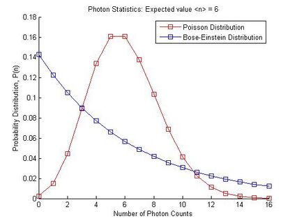
Comparison of the Poisson and Bose-Einstein distributions. The Poisson distribution is characteristic of coherent light while the Bose-Einstein distribution is characteristic of thermal light. Both distribution have the same expectation value [math]\displaystyle{ \langle n \rangle = 6 }[/math].

[math]\displaystyle{ I = \iint\limits_A \int_{t}^{t+\tau} \, I(x,y,t') dt'\,dx\,dy }[/math]

On substituting the intensity probability distribution of thermal light for P(I), Mandel's formula becomes

[math]\displaystyle{ P(n) = \int_{0}^{\infty} \frac{{\left ( \epsilon I \right )}^{n}}{n!} e^{-\epsilon I} \frac{e^{\frac{- I }{\langle I \rangle}}}{\langle I \rangle} dI = \frac{{\epsilon}^n}{n! \langle I \rangle} \int_{0}^{\infty} { I }^{n} e^{-\left ( \epsilon + \frac{1}{\langle I \rangle}\right )I} dI }[/math]

Using the following formula to evaluate the integral

[math]\displaystyle{ \int_{0}^{\infty} x^{n} e^{-ax} dx = \frac{n!}{a^{n+1}} \quad \left ( n = 0,1,2,.. a\gt 0\right) }[/math]

The probability distribution for n photon counts from a thermal light source is

[math]\displaystyle{ P(n) = \frac{1}{\left ( \langle n \rangle +1 \right )} {\left ( \frac{\langle n \rangle}{ \langle n \rangle +1}\right )}^n }[/math]

where [math]\displaystyle{ \langle n \rangle = \epsilon I }[/math] is the average number of counts. This last distribution is known as the Bose-Einstein distribution. The variance of the distribution can be shown to be

[math]\displaystyle{ {\Delta n }^2 = \langle n \rangle + {\langle n \rangle}^2 }[/math]

In contrast with the Poisson distribution for a coherent light source, the Bose-Einstein distribution has [math]\displaystyle{ {\Delta n}^2 \gt \langle n \rangle }[/math] characteristic of thermal light.

Sub-Poissonian light

Schematic of the homodyne intensity correlation scheme described in [6]. SI, signal field, LO, local oscillator, BS, beam splitter, SL, superimposed light, C, correlator. The photodetectors (black elements) send electrical signals to the correlator where the intensity correlation is measured.

Light that is governed by sub-Poisson statistics cannot be described by classical electromagnetic theory and is defined by [math]\displaystyle{ {\Delta n}^2 \lt \langle n \rangle }[/math]. The advent of ultrafast photodetectors has made it possible to measure the sub-Poissonian nature of light. An example of light exhibiting sub-Poissonian statistics is squeezed light. Recently researchers have shown that sub-Poissonian light can be induced in a quantum dot exhibiting resonance fluorescence. A technique used to measure the sub-Poissonian structure of light is a homodyne intensity correlation scheme. In this scheme a local oscillator and signal field are superimposed via a beam splitter. The superimposed light is then split by another beam splitter and each signal is recorded by individual photodetectors connected to correlator from which the intensity correlation can be measured. Evidence of the sub-Poissonian nature of light is shown by obtaining a negative intensity correlation as was shown in.

References

- ↑ 1.0 1.1 1.2 1.3 M. Fox, Quantum Optics: An Introduction, Oxford University Press, New York, 2006
- ↑ I. Deutsch, Quantum Optics Course Fall 2015, http://info.phys.unm.edu/~ideutsch/Classes/Phys566F15/Lectures/Phys566_Lect02.pdf. Retrieved 9 December 2015
- ↑ 3.0 3.1 Mandel, L (1959-09-01). "Fluctuations of Photon Beams: The Distribution of the Photo-Electrons". Proceedings of the Physical Society (IOP Publishing) 74 (3): 233–243. doi:10.1088/0370-1328/74/3/301. ISSN 0370-1328. Bibcode: 1959PPS....74..233M.
- ↑ J. W. Goodman, Statistical Optics, Wiley, New York, (1985) 238-256, 466-468
- ↑ 5.0 5.1 Schulte, Carsten H. H.; Hansom, Jack; Jones, Alex E.; Matthiesen, Clemens; Le Gall, Claire; Atatüre, Mete (2015-08-31). "Quadrature squeezed photons from a two-level system". Nature (Springer Science and Business Media LLC) 525 (7568): 222–225. doi:10.1038/nature14868. ISSN 0028-0836. PMID 26322581. Bibcode: 2015Natur.525..222S.
- ↑ Vogel, Werner (1995-05-01). "Homodyne correlation measurements with weak local oscillators". Physical Review A (American Physical Society (APS)) 51 (5): 4160–4171. doi:10.1103/physreva.51.4160. ISSN 1050-2947. PMID 9912091. Bibcode: 1995PhRvA..51.4160V.