Physics:Resonance fluorescence

Short description: Quantum electromechanical process

Resonance fluorescence is the process in which a two-level atom system interacts with the quantum electromagnetic field if the field is driven at a frequency near to the natural frequency of the atom.

General theory

Typically the photon contained electromagnetic field is applied to the two-level atom through the use of a monochromatic laser. A two-level atom is a specific type of two-state system in which the atom can be found in the two possible states. The two possible states are if an electron is found in its ground state or the excited state. In many experiments an atom of lithium is used because it can be closely modeled to a two-level atom as the excited states of the singular electron are separated by large enough energy gaps to significantly reduce the possibility of the electron jumping to a higher excited state. Thus it allows for easier frequency tuning of the applied laser as frequencies further off resonance can be used while still driving the electron to jump to only the first excited state. Once the atom is excited, it will release a photon with the same energy as the energy difference between the excited and ground state. The mechanism for this release is the spontaneous decay of the atom. The emitted photon is released in an arbitrary direction. While the transition between two specific energy levels is the dominant mechanism in resonance fluorescence, experimentally other transitions will play a very small role and thus must be taken into account when analyzing results. The other transitions will lead to emission of a photon of a different atomic transition with much lower energy which will lead to "dark" periods of resonance fluorescence.

The dynamics of the electromagnetic field of the monochromatic laser can be derived by first treating the two-level atom as a spin-1/2 system with two energy eigenstates which have energy separation of ħω₀. The dynamics of the atom can then be described by the three rotation operators, [math]\displaystyle{ \hat{R_{i}}(t) }[/math],[math]\displaystyle{ \hat{R_{j}}(t) }[/math],[math]\displaystyle{ \hat{R_{k}}(t) }[/math], acting upon the Bloch sphere. Thus the energy of the system is described entirely through an electric dipole interaction between the atom and field with the resulting hamiltonian being described by

[math]\displaystyle{ \hat{H} = \frac{1}{2}\int(\epsilon_{0}\hat{\vec{E}}^{2}(\vec{r},t)+\frac{1}{\mu_{0}}\hat{\vec{B}}^{2}(\vec{r},t))d^{3}x + \hbar \omega_{0} \hat{R_{k}}(t) + 2\omega_{0}\vec{\mu}\cdot\hat{\vec{A}}(0,t)\hat{R_{j}}(t) }[/math] .

After quantizing the electromagnetic field, the Heisenberg Equation as well as Maxwell's equations can then be used to find the resulting equations of motion for [math]\displaystyle{ \hat{R_{k}}(t) }[/math] as well as for [math]\displaystyle{ \hat{b}(t) }[/math], the annihilation operator of the field,

[math]\displaystyle{ \dot{\hat{R}}_{k}(t) = -2\beta(\hat{R}_{k}(t) + \frac{1}{2}) - (\omega_{0}/\hbar) \{[\hat{b}(t) +\hat{b}^{\dagger}(t)]\vec{\mu}\cdot\hat{\vec{A}}^{(+)}_{free}(\vec{r},t) + H.c.\} }[/math]

[math]\displaystyle{ \dot{\hat{b}}(t)=(-i\omega_{0}-\beta+i\gamma)\hat{b}(t)-(\beta + i \gamma)\hat{b}^{\dagger}(t)+2(\omega_{0}/\hbar)[\hat{R}_{k}(t)\vec{\mu}\cdot\hat{\vec{A}}^{(+)}_{free}(0,t) + H.c.] }[/math],

where [math]\displaystyle{ \beta }[/math] and [math]\displaystyle{ \gamma }[/math] are frequency parameters used to simplify equations.

Now that the dynamics of the field with respect to the states of the atom has been described, the mechanism through which photons are released from the atom as the electron falls from the excited state to the ground state, Spontaneous Emission, can be examined. Spontaneous emission is when an excited electron arbitrarily decays to the ground state emitting a photon. As the electromagnetic field is coupled to the state of the atom, and the atom can only absorb a single photon before having to decay, the most basic case then is if the field only contains a single photon. Thus spontaneous decay occurs when the excited state of the atom emits a photon back into the vacuum Fock state of the field [math]\displaystyle{ |e\rangle\otimes|\{0\}\rangle \Rightarrow |g\rangle\otimes|\{1\}\rangle }[/math]. During this process the decay of the expectation values of the above operators follow the following relations

[math]\displaystyle{ \langle \hat{R}_{k}(t)\rangle + \frac{1}{2} = [\langle\hat{R}_{k}(0)\rangle + \frac{1}{2}]e^{-2\beta t} }[/math],

[math]\displaystyle{ \langle\hat{b}_{s}(t)\rangle = \langle \hat{b}_{s}(0)\rangle e^{(-\beta + i\gamma)t} }[/math].

So the atom decays exponentially and the atomic dipole moment shall oscillate. The dipole moment oscillates due to the Lamb shift, which is a shift in the energy levels of the atom due to fluctuations of the field.

It is imperative, however, to look at fluorescence in the presence of a field with many photons, as this is a much more general case. This is the case in which the atom goes through many excitation cycles. In this case the exciting field emitted from the laser is in the form of coherent states [math]\displaystyle{ |\{v\}\rangle }[/math]. This allows for the operators which comprise the field to act on the coherent state and thus be replaced with eigenvalues. Thus we can simplify the equations by allowing operators to be turned into constants. The field can then be described much more classically than a quantized field normally would be able to. As a result, we are able to find the expectation value of the electric field for the retarded time.

[math]\displaystyle{ \langle \hat{\vec{E}}^{(-)}(\vec{r},t)\cdot \hat{\vec{E}}^{(+)}(\vec{r},t)\rangle = \left( \frac{\omega_{0}^{2}}{4\pi\epsilon_{0}c^{2}}\right)^{2} \left(\frac{\mu^{2}}{r^{2}} - \frac{(\vec{\mu}\cdot \vec{r})^{2}}{r^{4}}\right) \times \langle \hat{b}_{s}^{\dagger}\left( t-\frac{r}{c} \right) \hat{b}_{s}\left(t - \frac{r}{c}\right)\rangle = \left(\frac{\omega_{0}^{2} \mu \sin\psi}{4\pi\epsilon_{0}c^{2}r}\right)^{2}[\langle\hat{R}_{k}\left(t - \frac{r}{c}\right)\rangle + \frac{1}{2}] }[/math],

where [math]\displaystyle{ \psi }[/math] is the angle between [math]\displaystyle{ \hat{\mu} }[/math] and [math]\displaystyle{ \hat{r} }[/math].

There are two general types of excitations produced by fields. The first is one that dies out as [math]\displaystyle{ V = 0, t \Rightarrow \infty }[/math], while the other one reaches a state in which it eventually reaches a constant amplitude, thus [math]\displaystyle{ \hat{V}(t) = \hat{\epsilon}\alpha e^{i(\omega_{0}-\omega_{1})t+i\phi} }[/math].

Here [math]\displaystyle{ \alpha }[/math] is a real normalization constant, [math]\displaystyle{ \phi }[/math] is a real phase factor, and [math]\displaystyle{ \hat{\epsilon} }[/math] is a unit vector which indicates the direction of the excitation.

Thus as [math]\displaystyle{ t \Rightarrow \infty }[/math], then

[math]\displaystyle{ \langle \hat{R}_{k}(t)\rangle + 1/2 \Rightarrow \frac{\frac{1}{4}\Omega^{2}}{\frac{1}{2}\Omega^{2} + \beta^{2} + (\gamma + \omega_{1} - \omega_{0})^{2}} }[/math].

As [math]\displaystyle{ \Omega }[/math] is the Rabi frequency, we can see that this is analogous to the rotation of a spin state around the Bloch sphere from an interferometer. Thus the dynamics of a two-level atom can be accurately modeled by a photon in an interferometer. It is also possible to model as an atom and a field, and it will, in fact, retain more properties of the system such as lamb shift, but the basic dynamics of resonance fluorescence can be modeled as a spin-1/2 particle.

Resonance fluorescence in the Weak Field

There are several limits that can be analyzed to make the study of resonance fluorescence easier. The first of these is the approximations associated with the Weak Field Limit, where the square modulus of the Rabi frequency of the field that is coupled to two-level atom is much smaller than the rate of spontaneous emission of the atom. This means that the difference in the population between the excited state of the atom and the ground state of the atom is approximately independent of time. If we also take the limit in which the time period is much larger than the time for spontaneous decay, the coherences of the light can be modeled as [math]\displaystyle{ \rho_{ab}(t) = \frac{-i(\Omega_{R}/2)e^{-i\nu t}}{i(\omega - \nu) + \Gamma/2} [\rho_{aa}(0)-\rho_{bb}(0)] }[/math], where [math]\displaystyle{ \Omega_{R} }[/math] is the Rabi frequency of the driving field and [math]\displaystyle{ \Gamma }[/math] is the spontaneous decay rate of the atom. Thus it is clear that when an electric field is applied to the atom, the dipole of the atom oscillates according to driving frequency and not the natural frequency of the atom. If we also look at the positive frequency component of the electric field, [math]\displaystyle{ \langle \vec{E}^{(+)}(\vec{r},t)\rangle = \frac{\omega^{2}\mu \sin\psi}{4\pi\epsilon_{0}c^{2}|\vec{r}|} \hat{x} \langle \sigma_{-}(t-\frac{|\vec{r}|}{c})\rangle }[/math] we can see that the emitted field is the same as the absorbed field other than the difference in direction, resulting in the spectrum of the emitted field being the same as that of the absorbed field. The result is that the two-level atom behaves exactly as a driven oscillator and continues scattering photons so long as the driving field remains coupled to the atom.

The weak field approximation is also used in approaching two-time correlation functions. In the weak-field limit, the correlation function [math]\displaystyle{ \langle \hat{b}_{s}^{\dagger}(t)\hat{b}_{s}(t+\tau) \rangle }[/math] can be calculated much more easily as only the first three terms must be kept. Thus the correlation function becomes [math]\displaystyle{ \langle \hat{b}_{s}^{\dagger}(t)\hat{b}_{s}(t+\tau) \rangle = \frac{1}{4} \frac{\Omega^{2}e^{i(\omega_{0}-\omega_{1})\tau}}{\beta^{2}(1+\theta^{2})} \left (1-\frac{\Omega^{2}}{\frac{1}{2}\Omega^{2} + \beta^{2}(1+\theta^{2})} \right) + \frac{\Omega^{4}e^{-\beta|\tau|} e^{i(\omega_{0}-\omega_{1})\tau}}{8\beta^{4}\theta(1+\theta^{2})^{2}} \times [\sin(\beta\theta|\tau|) + \theta \cos(\beta\theta\tau)] }[/math] as [math]\displaystyle{ t \Rightarrow \infty }[/math].

From the above equation we can see that as [math]\displaystyle{ t \Rightarrow \infty }[/math] the correlation function will no longer depend on time, but rather that it will depend on [math]\displaystyle{ \tau }[/math]. The system will eventually reach a quasi-stationary state as [math]\displaystyle{ t \Rightarrow \infty }[/math] It is also clear that there are terms in the equation that go to zero as [math]\displaystyle{ \tau \Rightarrow \infty }[/math]. These are the result of the Markovian processes of the quantum fluctuations of the system. We see that in the weak field approximation as well as [math]\displaystyle{ t \Rightarrow \infty , \tau \Rightarrow \infty }[/math], the coupled system will reach a quasi-steady state where the quantum fluctuations become negligible.

Resonance fluorescence in the Strong Field

Schematic of a Mollet triplet

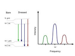
The Strong Field Limit is the exact opposite limit to the weak field where the square modulus of the Rabi frequency of the electromagnetic field is much larger than the rate of spontaneous emission of the two-level atom. When a strong field is applied to the atom, a single peak is no longer observed in fluorescent light's radiation spectrum. Instead, other peaks begin appearing on either side of the original peak. These are known as side bands. The sidebands are a result of the Rabi oscillations of the field causing a modulation in the dipole moment of the atom. This causes a splitting in the degeneracy of certain eigenstates of the hamiltonian, specifically [math]\displaystyle{ |e\rangle \otimes |\{n\}\rangle }[/math] and [math]\displaystyle{ |g\rangle \otimes |\{n+1\}\rangle }[/math] are split into doublets. This is known as dynamic Stark splitting and is the cause for the Mollow triplet, which is a characteristic energy spectrum found in Resonance fluorescence.

An interesting phenomena arises in the Mollow triplet where both of the sideband peaks have a width different than that of the central peak. If the Rabi frequency is allowed to become much larger than the rate of spontaneous decay of the atom, we can see that in the strong field limit [math]\displaystyle{ \langle \sigma_{-}(t)\rangle e^{i\omega t} }[/math] will become [math]\displaystyle{ \langle \sigma_{-}(t)\rangle e^{i\omega t} = \frac{1}{4} \{[2\rho_{++}(0)-1]e^{-\frac{\Gamma}{2}t} - [\rho_{+-}(0)e^{-i\Omega_{R}t-\frac{3\Gamma}{4}t}-c.c]\} }[/math]. From this equation it is clear where the differences in width of the peaks in the Mollow triplet arise from as the central peak has a width of [math]\displaystyle{ \frac{\Gamma}{2} }[/math] and the sideband peaks have a width of [math]\displaystyle{ \frac{3\Gamma}{4} }[/math] where [math]\displaystyle{ \Gamma }[/math] is the rate of spontaneous emission for the atom. Unfortunately this cannot be used to calculate a steady state solution as [math]\displaystyle{ \rho_{++}(0) \Rightarrow \frac{1}{2} }[/math] and [math]\displaystyle{ \rho_{+-}(0) \Rightarrow 0 }[/math] in a steady state solution. Thus the spectrum would vanish in a steady state solution, which is not the actual case.

The solution that does allow for a steady state solution must take the form of a two-time correlation function as opposed to the above one-time correlation function. This solution appears as

[math]\displaystyle{ \langle \sigma_{+}(0)\sigma_{-}(\tau)\rangle = \frac{1}{4} \left( e^{-\frac{\Gamma}{2}\tau} + \frac{1}{2}e^{-\frac{3\Gamma}{4}\tau}e^{-i\Omega_{R}\tau}+\frac{1}{2}e^{-\frac{3\Gamma}{4}\tau}e^{i\Omega_{R}\tau} \right) e^{-i\omega\tau} }[/math].

Since this correlation function includes the steady state limits of the density matrix, where [math]\displaystyle{ \rho_{++}^{s.s} \Rightarrow \frac{1}{2} }[/math] and [math]\displaystyle{ \rho_{+-}^{s.s} \Rightarrow 0 }[/math], and the spectrum is nonzero, it is clear to see that the Mollow triplet remains the spectrum for the fluoresced light even in a steady state solution.

General two-time correlation functions and spectral density

The study of correlation functions is critical to the study of quantum optics as the Fourier transform of the correlation function is the energy spectral density. Thus the two-time correlation function is a useful tool in the calculation of the energy spectrum for a given system. We take the parameter [math]\displaystyle{ \tau }[/math] to be the difference between the two times in which the function is calculated. While correlation functions can more easily be described using limits of the strength of the field and limits placed on the time of the system, they can be found more generally as well. For resonance fluorescence, the most important correlation functions are

[math]\displaystyle{ \langle \hat{b}_{s}^{\dagger}(t)\hat{b}_{s}(t+\tau)\rangle e^{i(\omega_{1}-\omega_{0})\tau} \equiv g(t,\tau) }[/math],

[math]\displaystyle{ \langle \hat{b}_{s}^{\dagger}(t)\hat{b}_{s}(t+\tau)\rangle e^{i(\omega_{1}-\omega_{0})(2t + \tau} e^{2i\phi} \equiv f(t,\tau) }[/math],

[math]\displaystyle{ \langle \hat{b}_{s}^{\dagger}(t)\hat{R}_{k}(t+\tau)\rangle e^{i(\omega_{1}-\omega_{0})t}e^{i\phi} \equiv g(t,\tau) }[/math],

where

[math]\displaystyle{ g(t,\tau) = [\langle \hat{R}_{k}(t)\rangle + \frac{1}{2}]e^{-\beta(1-i\theta)\tau} + \Omega \int\limits_{0}^{\tau} dt' h(t,t')e^{\beta(1-i\theta)(t'-\tau)} }[/math],

[math]\displaystyle{ f(t,\tau) = \Omega \int\limits_{0}^{\tau}dt' h(t,t')e^{\beta(1+i\theta)(t'-\tau)} }[/math],

[math]\displaystyle{ h(t,\tau) = -\frac{1}{2}\langle\hat{b}^{\dagger}_{s}(t)\rangle e^{i(\omega_{0} - \omega_{1})t}e^{i\phi} - \frac{1}{2}\Omega \int\limits_{0}^{\tau}dt'[f(t,t')+g(t,t')]e^{2\beta(t'-\tau)} }[/math].

Two-time correlation functions are generally shown to be independent of [math]\displaystyle{ t }[/math], and instead rely on [math]\displaystyle{ \tau }[/math] as [math]\displaystyle{ t \Rightarrow \infty }[/math]. These functions can be used to find the spectral density [math]\displaystyle{ S(t,\omega) }[/math] by computing the transform

[math]\displaystyle{ S (t,\omega) = K \int\limits_{0}^{\infty}d\tau g(t-\tau,\tau)e^{i(\omega - \omega_{1})\tau} + c.c }[/math],

where K is a constant. The spectral density can be viewed as the rate of photon emission of photons of frequency [math]\displaystyle{ \omega }[/math] at the given time [math]\displaystyle{ t }[/math], which is useful in determining the power output of a system at a given time.

The correlation function associated with the spectral density of resonance fluorescence is reliant on the electric field. Thus once the constant K has been determined, the result is equivalent to

[math]\displaystyle{ S(\vec{r},\omega_{0}) = \frac{1}{\pi} Re \int\limits_{0}^{\infty}d\tau\langle E^{(-)}(\vec{r},t)E^{(+)}(\vec{r},t+\tau)\rangle e^{i\omega_{0}\tau} }[/math]

This is related to the intensity by [math]\displaystyle{ \langle E^{(-)}(\vec{r},t)E^{(+)}(\vec{r},t+\tau)\rangle = I_{0}(\vec{r})\langle \sigma_{+}(t)\sigma_{-}(t+\tau)\rangle }[/math]

In the weak field limit when [math]\displaystyle{ \Omega_{R} \ll \frac{\Gamma}{4} }[/math] the power spectrum can be determined to be

[math]\displaystyle{ S(\vec{r},\omega_{0}) = I_{0}(\vec{r}) \left(\frac{\Omega_{R}}{\Gamma}\right)^{2} \delta(\omega-\omega_{0}) }[/math].

In the strong field limit, the power spectrum is slight more complicated and found to be

[math]\displaystyle{ S(\vec{r},\omega_{0}) = \frac{I_{0}(\vec{r})}{8\pi}\left[\frac{3\Gamma/4}{(\omega-\Omega_{R}-\omega_{0})^{2} + (3\Gamma/4)^{2}} + \frac{\Gamma}{(\omega-\omega_{0})^{2} + (\Gamma/2)^{2}} + \frac{3\Gamma/4}{(\omega + \Omega_{R}-\omega_{0})^{2} + (3\Gamma/4)^{2}} \right] }[/math].

From these two functions it is easy to see that in the weak field limit a single peak appears at [math]\displaystyle{ \omega_{0} }[/math] in the spectral density due to the delta function, while in the strong field limit a Mollow triplet forms with sideband peaks at [math]\displaystyle{ \omega = \omega_{0} \pm \Omega_{R} }[/math], and appropriate peak width of [math]\displaystyle{ \frac{\Gamma}{2} }[/math] for the central peak and [math]\displaystyle{ \frac{3\Gamma}{4} }[/math] for the sideband peaks.

Photon Anti-bunching

Photon anti-bunching is the process in Resonance Fluorescence through which rate at which photons are emitted by a two-level atom is limited. A two-level atom is only capable of absorbing a photon from the driving electromagnetic field after a certain period of time has passed. This time period is modeled as a probability distribution [math]\displaystyle{ p(\tau) }[/math] where [math]\displaystyle{ p(\tau) \Rightarrow 0 }[/math] as [math]\displaystyle{ \tau \Rightarrow 0 }[/math]. As the atom cannot absorb a photon, it is unable to emit one and thus there is a restriction on the spectral density. This is illustrated by the second order correlation function [math]\displaystyle{ g^{(2)}(\tau) = 1 - \left( cos\mu\tau + \frac{3\Gamma}{4\mu}sin\mu\tau \right) e^{-3\Gamma\tau/4} }[/math]. From the above equation it is clear that [math]\displaystyle{ g^{(2)}(0)=0 }[/math] and thus [math]\displaystyle{ g^{(2)}(\tau)\gt 0 }[/math] resulting in the relation that describes photon antibunching [math]\displaystyle{ g^{(2)}(\tau) \gt g^{(2)}(0) }[/math]. This shows that the power cannot be anything other than zero for [math]\displaystyle{ \tau = 0 }[/math]. In the weak field approximation [math]\displaystyle{ g^{(2)}(\tau) }[/math] can only increase monotonically as [math]\displaystyle{ \tau }[/math] increases, however in the strong field approximation [math]\displaystyle{ g^{(2)}(\tau) }[/math] oscillates as it increases. These oscillations die off as [math]\displaystyle{ \tau \Rightarrow \infty }[/math]. The physical idea behind photon anti-bunching is that while the atom itself is ready to be excited as soon as it releases its previous photon, the electromagnetic field created by the laser takes time to excite the atom.

Double Resonance

Double Resonance is the phenomena when an additional magnetic field is applied to a two-level atom in addition to the typical electromagnetic field used to drive resonance fluorescence. This lifts the spin degeneracy of the Zeeman energy levels splitting them along the energies associated with the respective available spin levels, allowing for not only resonance to be achieved around the typical excited state, but if a second driving electromagnetic associated with the Larmor frequency is applied, a second resonance can be achieved around the energy state associated with [math]\displaystyle{ m_{B} = 0 }[/math] and the states associated with [math]\displaystyle{ m_{b} = \pm 1 }[/math]. Thus resonance is achievable not only about the possible energy-levels of a two-level atom, but also about the sub-levels in the energy created by lifting the degeneracy of the level. If the applied magnetic field is tuned properly, the polarization of resonance fluorescence can be used to describe the composition of the excited state. Thus double resonance can be used to find the Landé factor, which is used to describe the magnetic moment of the electron within the two-level atom.

Resonance fluorescence of a single artificial atom

Any two state system can be modeled as a two-level atom. This leads to many systems being described as an "Artificial Atom". For instance a superconducting loop which can create a magnetic flux passing through it can act as an artificial atom as the current can induce a magnetic flux in either direction through the loop depending on whether the current is clockwise or counterclockwise. The hamiltonian for this system is described as [math]\displaystyle{ \hat{H} = \hbar \sqrt{\omega^{2}_{0} + \epsilon^{2}}\frac{\hat{\sigma}_{z}}{2} }[/math] where [math]\displaystyle{ \hbar \epsilon = 2I_{p}\delta\Phi }[/math]. This models the dipole interaction of the atom with a 1-D electromagnetic wave. It is easy to see that this is truly analogous to a real two-level atom due to the fact that the fluorescence appears in the spectrum as the Mollow triplet, precisely like a true two-level atom. These artificial atoms are often used to explore the phenomena of quantum coherence. This allows for the study of squeezed light which is known for creating more precise measurements. It is difficult to explore the resonance fluorescence of squeezed light in a typical two-level atom as all modes of the electromagnetic field must be squeezed which cannot easily be accomplished. In an artificial atom, the number of possible modes of the field is significantly limited allowing for easier study of squeezed light. In 2016 D.M. Toyli et al., performed an experiment in which two superconducting parametric amplifiers were used to generate squeezed light and then detect resonance fluorescence in artificial atoms from the squeezed light. Their results agreed strongly with the theory describing the phenomena. The implication of this study is it allows for resonance fluorescence to assist in qubit readout for squeezed light. The qubit used in the study was an aluminum transmon circuit that was then coupled to a 3-D aluminum cavity. Extra silicon chips were introduced to the cavity to assist in the tuning of resonance to that of the cavity. The majority of the detuning that did occur was a result of the degeneration of the qubit over time.

Resonance fluorescence from a Semiconductor Quantum Dot

A quantum dot is a semiconductor nano-particle that is often used in quantum optical systems. This includes their ability to be placed in optical microcavities where they can act as two-level systems. In this process, quantum dots are placed in cavities which allow for the discretization of the possible energy states of the quantum dot coupled with the vacuum field. The vacuum field is then replaced by an excitation field and resonance fluorescence is observed. Current technology only allows for population of the dot in an excited state (not necessarily always the same), and relaxation of the quantum dot back to its ground state. Direct excitation followed by ground state collection was not achieved until recently. This is mainly due to the fact that as a result of the size of quantum dots, defects and contaminants create fluorescence of their own apart from the quantum dot. This desired manipulation has been achieved by quantum dots by themselves through a number of techniques including four-wave mixing and differential reflectivity, however no techniques had shown it to occur in cavities until 2007. Resonance fluorescence has been seen in a single self-assembled quantum dot as presented by Muller among others in 2007. In the experiment they used quantum dots that were grown between two mirrors in the cavity. Thus the quantum dot was not placed in the cavity, but instead created in it. They then coupled a strong in-plane polarized tunable continuous-wave laser to the quantum dot and were able to observe resonance fluorescence from the quantum dot. In addition to the excitation of the quantum dot that was achieved, they were also able to collect the photon that was emitted with a micro-PL setup. This allows for resonant coherent control of the ground state of the quantum dot while also collecting the photons emitted from the fluorescence.

Coupling photons to a molecule

In 2007, G. Wrigge, I. Gerhardt, J. Hwang, G. Zumofen, and V. Sandoghdar developed an efficient method to observe resonance fluorescence for an entire molecule as opposed to its typical observation in a single atom. Instead of coupling the electric field to a single atom, they were able to replicate two-level systems in dye molecules embedded in solids. They used a tunable dye laser to excite the dye molecules in their sample. Due to the fact that they could only have one source at a time, the proportion of shot noise to actual data was much higher than normal. The sample which they excited was a Shpol'skii matrix which they had doped with the dyes they wished to use, dibenzanthanthrene. To improve the accuracy of the results, single-molecule fluorescence-excitation spectroscopy was used. The actual process for measuring the resonance was measuring the interference between the laser beam and the photons that were scattered from the molecule. Thus the laser was passed over the sample, resulting in several photons were scattered back, allowing for the measurement of the interference in the electromagnetic field that resulted. The improvement to this technique was they used solid-immersion lens technology. This is a lens that has a much higher numerical aperture than normal lenses as it is filled with a material that has a large refractive index. The technique used to measure the resonance fluorescence in this system was originally designed to locate individual molecules within substances.

Implications of Resonance fluorescence

The largest implication that arises from resonance fluorescence is that for future technologies. Resonance fluorescence is used primarily in the coherent control of atoms. By coupling a two-level atom, such as a quantum dot, to an electric field in the form of a laser, you are able to effectively create a qubit. The qubit states correspond to the excited and the ground state of the two-level atoms. Manipulation of the electromagnetic field allows for effective control of the dynamics of the atom. These can then be used to created quantum computers. The largest barriers that still stand in the way of this being achievable are failures in truly controlling the atom. For instance true control of spontaneous decay and decoherence of the field pose large problems that must be overcome before two-level atoms can truly be used as qubits.

References

- ↑ H.J. Kimble; L. Mandel (June 1976). "Theory of resonance fluorescence". Physical Review A 13 (6): 2123–2144. doi:10.1103/PhysRevA.13.2123. Bibcode: 1976PhRvA..13.2123K. https://journals.aps.org/pra/abstract/10.1103/PhysRevA.13.2123.
- ↑ Harry Paul (2004). Introduction to Quantum Optics. The Edinburgh Building, Cambridge cb2 2ru, UK: Cambridge University Press. pp. 61–63. ISBN 978-0-521-83563-3. https://archive.org/details/introductiontoqu0000paul.
- ↑ Marlan O. Scully; M. Suhail Zubairy (1997). Quantum Optics (1 ed.). The Pitt Building, Cambridge CB2 2RU, UK: Cambridge University Press. pp. 291–327. ISBN 0-521-43458-0. https://archive.org/details/quantumoptics00scul_728.
- ↑ Gilbert Grynberg; Alain Aspect; Claude Fabre (2010). Introduction to Quantum Optics. Cambridge, UK: Cambridge University Press. pp. 120–140. ISBN 978-0-521-55112-0. https://archive.org/details/introductiontoqu00gryn.
- ↑ O. Astafiev; A.M. Zagoskin; A.A. Abdumalikov Jr.; Yu. A. Pashkin; T. Yamamoto; K. Inomata; Y. Makamura; J.S. Tsai (12 Feb 2010). "Resonance Fluorescence of a Single Artificial Atom". Science 327 (5967): 840–843. doi:10.1126/science.1181918. PMID 20150495. Bibcode: 2010Sci...327..840A.
- ↑ D.M. Toyli; A.W. Eddins; S. Boutin; S. Puri; D. Hover; V. Bolkhovsky; W.D. Oliver; A. Blais et al. (11 July 2016). "Resonance Fluorescence from an Artificial Atom in Squeezed Vacuum". Physical Review X 6 (3). doi:10.1103/PhysRevX.6.031004. Bibcode: 2016PhRvX...6c1004T.
- ↑ A. Muller; E. B. Flagg; P. Bianucci; X.Y. Wang; D.G. Deppe; W. Ma; J. Zhang; G.J. Salamo et al. (1 November 2007). "Resonance Fluorescence from a Coherently Driven Semiconductor Quantum Dot in a Cavity". Physical Review Letters 99 (18). doi:10.1103/PhysRevLett.99.187402. PMID 17995437. Bibcode: 2007PhRvL..99r7402M.
- ↑ G. Wrigge; I. Gerhardt; J. Hwang; G. Zumofen; V. Sandoghdar (16 December 2007). "Efficient coupling of photons to a single molecule and the observation of its resonance fluorescence". Nature 4 (1): 60–66. doi:10.1038/nphys812. Bibcode: 2008NatPh...4...60W.