Physics:Stoner–Wohlfarth model

The Stoner–Wohlfarth model is a widely used model for the magnetization of single-domain ferromagnets. It is a simple example of magnetic hysteresis and is useful for modeling small magnetic particles in magnetic storage, biomagnetism, rock magnetism and paleomagnetism.

History

The Stoner–Wohlfarth model was developed by Edmund Clifton Stoner and Erich Peter Wohlfarth and published in 1948. It included a numerical calculation of the integrated response of randomly oriented magnets. Since this was done before computers were widely available, they resorted to trigonometric tables and hand calculations.

Description

Figure 1. Illustration of the variables used in the Stoner–Wolhfarth model. The dashed line is the easy axis of the particle.

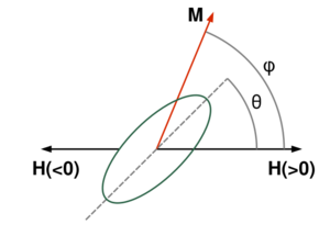
In the Stoner–Wohlfarth model, the magnetization does not vary within the ferromagnet and it is represented by a vector M. This vector rotates as the magnetic field H changes. The magnetic field is only varied along a single axis; its scalar value h is positive in one direction and negative in the opposite direction. The ferromagnet is assumed to have a uniaxial magnetic anisotropy with anisotropy parameter K_u. As the magnetic field varies, the magnetization is restricted to the plane containing the magnetic field direction and the easy axis. It can therefore be represented by a single angle φ, the angle between the magnetization and the field (Figure 1). Also specified is the angle θ between the field and the easy axis.

Equations

The energy of the system is

[math]\displaystyle{ E = K_uV\sin^2\left(\varphi-\theta\right) - \mu_0M_sVH\cos\varphi, \, }[/math]

(1)

where V is the volume of the magnet, M_s is the saturation magnetization, and μ₀ is the vacuum permeability. The first term is the magnetic anisotropy and the second the energy of coupling with the applied field (often called the Zeeman energy).

Stoner and Wohlfarth normalized this equation:

[math]\displaystyle{ \eta = \frac{E}{2K_uV} = \frac{1}{4} -\frac{1}{4}\cos\left(2\left(\varphi-\theta\right)\right) - h\cos\varphi, \, }[/math]

(2)

where h = μ₀M_sH/2K_u. A given magnetization direction is in mechanical equilibrium if the forces on it are zero. This occurs when the first derivative of the energy with respect to the magnetization direction is zero:

[math]\displaystyle{ \frac{\partial\eta}{\partial \varphi} = \frac{1}{2}\sin\left(2\left(\varphi-\theta\right)\right) + h\sin\varphi = 0. \, }[/math]

(3)

This direction is stable against perturbations when it is at an energy minimum, having a positive second derivative:

[math]\displaystyle{ \frac{\partial^2\eta}{\partial \varphi^2} = \cos\left(2\left(\varphi-\theta\right)\right) + h\cos\varphi \gt 0. \, }[/math]

(4)

In zero field the magnetic anisotropy term is minimized when the magnetization is aligned with the easy axis. In a large field, the magnetization is pointed towards the field.

Hysteresis loops

Figure 2. An example solution of the Stoner–Wolhfarth model. Both h and m_h are between −1 and +1. The solid red and blue curves are energy minima, the dashed red and blue lines are energy maxima. Energy profiles are included for three vertical profiles (insets).

For each angle θ between easy axis and field, equation (3) has a solution that consists of two solution curves. It is trivial to solve for these curves by varying φ and solving for h. There is one curve for φ between 0 and π and another for φ between π and 2π; the solutions at φ = 0 and π correspond to h = ±∞.

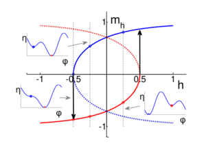
Since the magnetization in the direction of the field is M_s cos φ, these curves are usually plotted in the normalized form m_h vs. h, where m_h = cos φ is the component of magnetization in the direction of the field. An example is shown in Figure 2. The solid red and blue curves connect stable magnetization directions. For fields −1/2 ≤ h ≤ 1/2, the two curves overlap and there are two stable directions. This is the region where hysteresis occurs. Three energy profiles are included (insets). The red and blue stars are the stable magnetization directions, corresponding to energy minima. Where the vertical dashed lines intersect the red and blue dashed lines, the magnetization directions are energy maxima and determine the energy barriers between states.

In an ordinary magnetic hysteresis measurement, h starts at a large positive value and is decreased to a large negative value. The magnetization direction starts on the blue curve. At h = 0.5 the red curve appears, but for h > 0 the blue state has a lower energy because it is closer to the direction of the magnetic field. When the field becomes negative, the red state has the lower energy, but the magnetization cannot immediately jump to this new direction because there is an energy barrier in between (see the insets). At h = −0.5, however, the energy barrier disappears, and in more negative fields the blue state no longer exists. It must therefore jump to the red state. After this jump, the magnetization remains on the red curve until the field increases past h = 0.5, where it jumps to the blue curve. Usually only the hysteresis loop is plotted; the energy maxima are only of interest if the effect of thermal fluctuations is calculated.

The Stoner–Wohlfarth model is a classic example of magnetic hysteresis. The loop is symmetric (by a 180^° rotation) about the origin and jumps occur at h = ± h_s, where h_s is known as the switching field. All the hysteresis occurs at ± h_s.

Dependence on field direction

Figure 3. Some hysteresis loops predicted by the Stoner–Wolhfarth model for different angles (θ) between the field and easy axis.

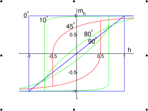
The shape of the hysteresis loop has a strong dependence on the angle between the magnetic field and the easy axis (Figure 3). If the two are parallel (θ = 0), the hysteresis loop is at its biggest (with m_h = h_s = 1 in normalized units). The magnetization starts parallel to the field and does not rotate until it becomes unstable and jumps to the opposite direction. In general, the larger the angle, the more reversible rotation occurs. At the other extreme of θ = 90^°, with the field perpendicular to the easy axis, no jump occurs. The magnetization rotates continuously from one direction to the other (it has two choices of rotation direction, though).

For a given angle θ, the switching field is the point where the solution switches from an energy minimum (∂²η/∂ φ² > 0) to an energy maximum (∂²η/∂ φ² < 0). Thus, it can be calculated directly by solving equation (3) along with ∂²η/∂ φ² = 0. The solution is

[math]\displaystyle{ h_s = \frac{\left(1-t^2+t^4\right)^{1/2}}{1+t^2}, \, }[/math]

(5)

where

[math]\displaystyle{ t=\tan^{1/3}\theta. \, }[/math]

(6)

In normalized units, 0.5 ≤ h_s ≤ 1.

An alternative way of representing the switching field solution is to divide the vector field h into a component h_|| = h cos θ that is parallel to the easy axis, and a component h_⊥ = h sin θ that is perpendicular. Then

[math]\displaystyle{ h_\parallel^{2/3}+h_\perp^{2/3}=1. \, }[/math]

(7)

If the components are plotted against each other, the result is a Stoner–Wohlfarth astroid. A magnetic hysteresis loop can be calculated by applying a geometric construction to this astroid.

Predictions for homogeneous, isotropic systems

Hysteresis

Figure 4. Main hysteresis loop for an isotropic sample with identical particles. The magnetization and field are normalized (m_h = M_H/M_s, h = H/2K_u). The curve starting at the origin is the initial magnetization curve. Double arrows represent reversible change, a single arrow irreversible change.

Stoner and Wohlfarth calculated the main hysteresis loop for an isotropic system of randomly oriented, identical particles. The result of the calculation is reproduced in Figure 4. Irreversible change (single arrow) occurs for 0.5 < |h| < 1, reversible change (double arrows) elsewhere. The normalized saturation remanence m_rs and coercivity h_c are indicated on the figure. The curve in the center is the initial magnetization curve. This simulates the behavior of the sample if it is demagnetized before applying a field. The demagnetization is assumed to leave each particle with an equal probability of being magnetized in either of the two directions parallel to the easy axis. Thus, it is an average of the upper and lower branches of the main loop.

Isothermal remanence

Figure 5. Three kinds of isothermal remanence for an isotropic system of randomly oriented, identical particles. The remanences are m_ir, isothermal remanent magnetization; m_af, alternating field demagnetization remanence; and m_df, dc demagnetization remanence.

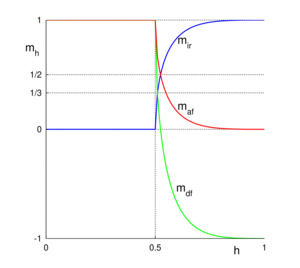
Some remanence calculations for randomly oriented, identical particles are shown in Figure 5. Isothermal remanent magnetization (IRM) is acquired after demagnetizing the sample and then applying a field. The curve m_ir(h) shows the normalized remanence as a function of the field. No change occurs until h = 0.5 because all the switching fields are larger than 0.5. Up to this field, changes in magnetization are reversible. The magnetization reaches saturation at h = 1, the largest switching field.

The other two types of remanence involve demagnetizing a saturation isothermal remanence (SIRM), so in normalized units they start at 1. Again, nothing happens to the remanence until the field reaches 0.5. The field at which m_dc reaches zero is called the coercivity of remanence.

Hysteresis parameters predicted for identical, randomly oriented particles

Parameter	Prediction
[math]\displaystyle{ M_{rs}/M_s }[/math]	[math]\displaystyle{ 0.5 }[/math]
[math]\displaystyle{ H_c/2K_u }[/math]	[math]\displaystyle{ 0.479 }[/math]
[math]\displaystyle{ H_{cr}/2K_u }[/math]	[math]\displaystyle{ 0.524 }[/math]
[math]\displaystyle{ \chi_0/2K_u }[/math]	[math]\displaystyle{ 2/3 }[/math]
[math]\displaystyle{ H_{cr}/H_c }[/math]	[math]\displaystyle{ 1.09 }[/math]

Some magnetic hysteresis parameters predicted by this calculation are shown in the adjacent table. The normalized quantities used in the above equations have been expressed in terms of the normal measured quantities. The parameter H_cr is the coercivity of remanence and χ₀ is the initial susceptibility (the magnetic susceptibility of a demagnetized sample).

More general systems

The above calculations are for identical particles. In a real sample the magnetic anisotropy parameter K_u will be different for each particle. This does not change the ratio M_rs/M_s, but it does change the overall shape of the loop. A parameter that is often used to characterize the shape of the loop is the ratio H_cr/H_c, which is 1.09 for a sample with identical particles and larger if they are not identical. Plots of M_rs/M_s against H_cr/H_c are widely used in rock magnetism as a measure of the domain state (single-domain or multidomain) in magnetic minerals.

Wohlfarth relations

Wohlfarth identified relations between the remanences that hold true for any system of Stoner–Wohlfarth particles:

[math]\displaystyle{ \begin{align} M_{af}(H) &= M_{rs} - M_{ir}(H) \\ M_{df}(H) &= M_{rs} - 2M_{ir}(H) \end{align}. \, }[/math]

(8)

These Wohlfarth relations compare IRM with demagnetization of saturation remanence. Wohlfarth also described more general relations comparing the acquiring a non-saturation IRM and demagnetizing it.

The Wohlfarth relations can be represented by linear plots of one remanence against another. These Henkel plots are often used to display measured remanence curves of real samples and determine whether Stoner–Wohlfarth theory applies to them.

Extensions of the model

The Stoner–Wohlfarth model is useful in part because it is so simple, but it often falls short of representing the actual magnetic properties of a magnet. There are several ways in which it has been extended:

• Generalizing the magnetic anisotropy: Hysteresis loops have been calculated for particles with pure cubic magnetocrystalline anisotropy as well as mixtures of cubic and uniaxial anisotropy.
• Adding thermal fluctuations: Thermal fluctuations make jumps between stable states possible, reducing the hysteresis in the system. Pfeiffer added the effect of thermal fluctuations to the Stoner–Wohlfarth model. This makes the hysteresis dependent on the size of the magnetic particle. As the particle size (and the time between jumps) decreases, it eventually crosses over into superparamagnetism.
• Adding particle interactions: Magnetostatic or exchange coupling between magnets can have a large effect on the magnetic properties. If the magnets are in a chain, they may act in unison, behaving much like Stoner–Wohlfarth particles. This effect is seen in the magnetosomes of magnetotactic bacteria. In other arrangements, the interactions may reduce the hysteresis.
• Generalizing to non-uniform magnetization: This is the domain of micromagnetics.

See also

• Stoner–Wohlfarth astroid

References

• Day, R.; Fuller, M.; Schmidt, V. A. (1977). "Hysteresis properties of titanomagnetites: grain-size and compositional dependence". Physics of the Earth and Planetary Interiors 13 (4): 260–267. doi:10.1016/0031-9201(77)90108-X. Bibcode: 1977PEPI...13..260D. 
• Mayergoyz, Isaak D. (2003). Mathematical Models of Hysteresis and their Applications (Second ed.). Academic Press. ISBN 978-0124808737. 
• Pfeiffer, H. (1990). "Determination of anisotropy field distribution in particle assemblies taking into account thermal fluctuations". Physica Status Solidi A 118 (1): 295–306. doi:10.1002/pssa.2211180133. Bibcode: 1990PSSAR.118..295P. 
• Stoner, E. C.; Wohlfarth, E. P. (1948). "A mechanism of magnetic hysteresis in heterogeneous alloys". Philosophical Transactions of the Royal Society A: Mathematical, Physical and Engineering Sciences 240 (826): 599–642. doi:10.1098/rsta.1948.0007. Bibcode: 1948RSPTA.240..599S. 
• Wohlfarth, E. P. (1958). "Relations between different modes of acquisition of the remanent magnetization of ferromagnetic particles". Journal of Applied Physics 29 (3): 595–596. doi:10.1063/1.1723232. Bibcode: 1958JAP....29..595W. 
• Zhang, H.; Rong, C.; Zhang, J.; Zhang, S.; Zhang, Shao-Ying; Shen, Bao-gen (2003). "Investigation on intergrain exchange coupling of nanocrystalline permanent magnets by Henkel plot". Applied Physics Letters 82 (23): 4098–4100. doi:10.1063/1.1576291. Bibcode: 2003ApPhL..82.4098Z. 

External links

• Stoner-Wohlfarth magnetization reversal app