Piecewise linear continuation

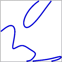
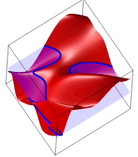
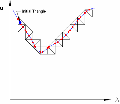
Simplicial continuation, or piecewise linear continuation (Allgower and Georg), is a one-parameter continuation method which is well suited to small to medium embedding spaces. The algorithm has been generalized to compute higher-dimensional manifolds by (Allgower and Gnutzman) and (Allgower and Schmidt). The algorithm for drawing contours is a simplicial continuation algorithm, and since it is easy to visualize, it serves as a good introduction to the algorithm.

Contour plotting

The contour plotting problem is to find the zeros (contours) of [math]\displaystyle{ f(x,y)=0\, }[/math] ([math]\displaystyle{ f(\cdot)\, }[/math] a smooth scalar valued function) in the square [math]\displaystyle{ 0\leq x \leq 1, 0\leq y \leq 1\, }[/math],

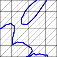
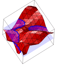
The square is divided into small triangles, usually by introducing points at the corners of a regular square mesh [math]\displaystyle{ ih_x\leq x\leq (i+1)h_x\, }[/math], [math]\displaystyle{ jh_y\leq y \leq (j+1)h_y\, }[/math], making a table of the values of [math]\displaystyle{ f(x_i,y_j)\, }[/math] at each corner [math]\displaystyle{ (i,j)\, }[/math], and then dividing each square into two triangles. The value of [math]\displaystyle{ f(x_i,y_j)\, }[/math] at the corners of the triangle defines a unique Piecewise Linear interpolant [math]\displaystyle{ lf(x,y)\, }[/math] to [math]\displaystyle{ f(\cdot)\, }[/math] over each triangle. One way of writing this interpolant on the triangle with corners [math]\displaystyle{ (x_0,y_0),~(x_1,y_1),~(x_2,y_2)\, }[/math] is as the set of equations

[math]\displaystyle{ (x,y) = (x_0,y_0)+(x_1-x_0,y_1-y_0)s+(x_2-x_0,y_2-y_0)t\, }[/math]

[math]\displaystyle{ 0\leq s\, }[/math]

[math]\displaystyle{ 0\leq t\, }[/math]

[math]\displaystyle{ s+t \leq 1\, }[/math]

[math]\displaystyle{ lf(x,y) = f(x_0,y_0)+(f(x_1,y_1)-f(x_0,y_0))s+(f(x_2,y_2)-f(x_0,y_0))t\, }[/math]

The first four equations can be solved for [math]\displaystyle{ (s,t)\, }[/math] (this maps the original triangle to a right unit triangle), then the remaining equation gives the interpolated value of [math]\displaystyle{ f(\cdot)\, }[/math]. Over the whole mesh of triangles, this piecewise linear interpolant is continuous.

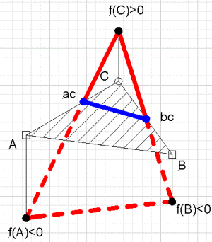
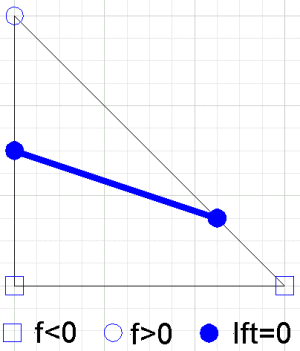
The contour of the interpolant on an individual triangle is a line segment (it is an interval on the intersection of two planes). The equation for the line can be found, however the points where the line crosses the edges of the triangle are the endpoints of the line segment.

The contour of the piecewise linear interpolant is a set of curves made up of these line segments. Any point on the edge connecting [math]\displaystyle{ (x_0,y_0)\, }[/math] and [math]\displaystyle{ (x_1,y_1)\, }[/math] can be written as

[math]\displaystyle{ (x,y) = (x_0,y_0) + t (x_1-x_0,y_1-y_0),\, }[/math]

with [math]\displaystyle{ t\, }[/math] in [math]\displaystyle{ (0,1)\, }[/math], and the linear interpolant over the edge is

[math]\displaystyle{ f \sim f_0 + t (f_1-f_0)\, }[/math]

So setting [math]\displaystyle{ f = 0\, }[/math]

[math]\displaystyle{ t = -f_0/(f_1-f_0)\, }[/math] and [math]\displaystyle{ (x,y) = (x_0,y_0)-f_0*(x_1-x_0,y_1-y_0)/(f_1-f_0)\, }[/math]

Since this only depends on values on the edge, every triangle which shares this edge will produce the same point, so the contour will be continuous. Each triangle can be tested independently, and if all are checked the entire set of contour curves can be found.

Piecewise linear continuation

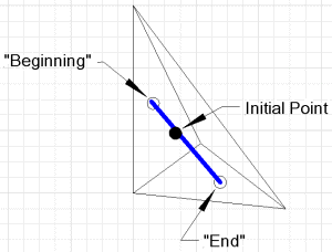
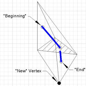
Piecewise linear continuation is similar to contour plotting (Dobkin, Levy, Thurston and Wilks), but in higher dimensions. The algorithm is based on the following results:

Lemma 1

If F(x) maps [math]\displaystyle{ \mathbb{R}^n }[/math] into [math]\displaystyle{ \mathbb{R}^{n-1} }[/math], there is a unique linear interpolant on an '(n-1)'-dimensional simplex which agrees with the function values at the vertices of the simplex.

An '(n-1)'-dimensional simplex has n vertices, and the function F assigns an 'n'-vector to each. The simplex is convex, and any point within the simplex is a convex combination of the vertices. That is:

If x is in the interior of an (n-1)-dimensional simplex with n vertices [math]\displaystyle{ v_i }[/math], then there are positive scalars [math]\displaystyle{ 0\lt \alpha_i }[/math] such that

[math]\displaystyle{ \mathbf{x} = \sum_i \alpha_i \mathbf{v}_i }[/math]

[math]\displaystyle{ \sum_i \alpha_i = 1.\, }[/math]

If the vertices of the simplex are linearly independent the non-negative scalars [math]\displaystyle{ \alpha }[/math] are unique for each point x, and are called the barycentric coordinates of x. They determine the value of the unique interpolant by the formula:

[math]\displaystyle{ LF = \sum_i \alpha_i F(\mathbf{v}_i) }[/math]

Lemma 2

An (n-1)-dimensional simplex can be tested to determine if it contains the origin.

There are basically two tests. The one which was first used labels the vertices of the simplex with a vector of signs (+/-) of the coordinates of the vertex. For example the vertex (.5,-.2,1.) would be labelled (+,-,+). A simplex is called completely labelled if there is a vertex whose label begins with a string of "+" signs of length 0,1,2,3,4,...n. A completely labelled simplex contains a neighborhood of the origin. This may be surprising, but what underlies this result is that for each coordinate of a completely labelled simplex there is a vector with "+" and another with a "-". Put another way, the smallest cube with edges parallel to the coordinate axes and which covers the simplex has pairs of faces on opposite sides of 0. (i.e. a "+" and a "-" for each coordinate).

The second approach is called vector labelling. It is based on the barycentric coordinates of the vertices of the simplex. The first step is to find the barycentric coordinates of the origin, and then the test that the simplex contains the origin is simply that all the barycentric coordinates are positive and the sum is less than 1.

Lemma 3

There is a triangulation (the Coxeter-Freudenthal-Kuhn triangulation [1]) which is invariant under the pivot operation [math]\displaystyle{ P_{v_i} (v_0,v_1,...,v_n) := (v_0,v_1,...,v_{i-1},\tilde v_i,v_{i+1},...,v_n) }[/math] where [math]\displaystyle{ \tilde v_i = \left\{ \begin{array}{lcl} v_1+v_n-v_0 & &i=0 \\ v_{i+1}+v_{i-1}-v_i&\qquad\qquad&0\\ v_{n-1}+v_0-v_n & &i=n \\ \end{array}\right. }[/math]

References

- ↑ Eugene L. Allgower, K. Georg, "Introduction to Numerical Continuation Methods", SIAM Classics in Applied Mathematics 45, 2003.
- ↑ E. L. Allgower, K. Georg, "Simplicial and Continuation Methods for Approximating Fixed Points and Solutions to Systems of Equations", SIAM Review, Volume 22, 28-85, 1980.
- ↑ Eugene L. Allgower, Stefan Gnutzmann, "An Algorithm for Piecewise Linear Approximation of Implicitly Defined Two-Dimensional Surfaces", SIAM Journal on Numerical Analysis, Volume 24, Number 2, 452-469, 1987.
- ↑ Eugene L. Allgower, Phillip H. Schmidt, "An Algorithm for Piecewise-Linear Approximation of an Implicitly Defined Manifold", SIAM Journal on Numerical Analysis, Volume 22, Number 2, 322-346, April 1985.
- ↑ David P. Dobkin, Silvio V. F. Levy, William P. Thurston and Allan R. Wilks, "Contour Tracing by Piecewise Linear Approximations", ACM Transactions on Graphics, 9(4) 389-423, 1990.