Prony's method

Short description: Method to estimate the components of a signal

Prony analysis of a time-domain signal

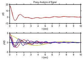
Prony analysis (Prony's method) was developed by Gaspard Riche de Prony in 1795. However, practical use of the method awaited the digital computer. Similar to the Fourier transform, Prony's method extracts valuable information from a uniformly sampled signal and builds a series of damped complex exponentials or damped sinusoids. This allows the estimation of frequency, amplitude, phase and damping components of a signal.

The method

Let [math]\displaystyle{ f(t) }[/math] be a signal consisting of [math]\displaystyle{ N }[/math] evenly spaced samples. Prony's method fits a function

[math]\displaystyle{ \hat{f}(t) = \sum_{i=1}^{N} A_i e^{\sigma_i t} \cos(\omega_i t + \phi_i) }[/math]

to the observed [math]\displaystyle{ f(t) }[/math]. After some manipulation utilizing Euler's formula, the following result is obtained, which allows more direct computation of terms:

[math]\displaystyle{ \begin{align} \hat{f}(t) &= \sum_{i=1}^{N} A_i e^{\sigma_i t} \cos(\omega_i t + \phi_i) \\ &= \sum_{i=1}^{N} \frac{1}{2} A_i \left( e^{j\phi_i}e^{\lambda^+_i t} + e^{-j\phi_i}e^{\lambda^-_i t}\right), \end{align} }[/math]

where

[math]\displaystyle{ \lambda^{\pm}_i = \sigma_i \pm j \omega_i }[/math] are the eigenvalues of the system,

[math]\displaystyle{ \sigma_i = -\omega_{0,i} \xi_i }[/math] are the damping components,

[math]\displaystyle{ \omega_i = \omega_{0,i} \sqrt{1-\xi_i^2} }[/math] are the angular-frequency components,

[math]\displaystyle{ \phi_i }[/math] are the phase components,

[math]\displaystyle{ A_i }[/math] are the amplitude components of the series,

[math]\displaystyle{ j }[/math] is the imaginary unit ([math]\displaystyle{ j^2 = -1 }[/math]).

Representations

Prony's method is essentially a decomposition of a signal with [math]\displaystyle{ M }[/math] complex exponentials via the following process:

Regularly sample [math]\displaystyle{ \hat{f}(t) }[/math] so that the [math]\displaystyle{ n }[/math]-th of [math]\displaystyle{ N }[/math] samples may be written as

[math]\displaystyle{ F_n = \hat{f}(\Delta_t n) = \sum_{m=1}^{M} \Beta_m e^{\lambda_m \Delta_t n}, \quad n=0,\dots,N-1. }[/math]

If [math]\displaystyle{ \hat{f}(t) }[/math] happens to consist of damped sinusoids, then there will be pairs of complex exponentials such that

[math]\displaystyle{ \begin{align} \Beta_a &= \frac{1}{2} A_i e^{ \phi_i j}, \\ \Beta_b &= \frac{1}{2} A_i e^{-\phi_i j}, \\ \lambda_a &= \sigma_i + j \omega_i, \\ \lambda_b &= \sigma_i - j \omega_i, \end{align} }[/math]

where

[math]\displaystyle{ \begin{align} \Beta_a e^{\lambda_a t} + \Beta_b e^{\lambda_b t} &= \frac{1}{2} A_i e^{\phi_i j} e^{(\sigma_i + j \omega_i) t} + \frac{1}{2}A_i e^{-\phi_i j} e^{(\sigma_i - j \omega_i) t} \\ &= A_i e^{\sigma_i t} \cos(\omega_i t + \phi_i). \end{align} }[/math]

Because the summation of complex exponentials is the homogeneous solution to a linear difference equation, the following difference equation will exist:

[math]\displaystyle{ \hat{f}(\Delta_t n) = \sum_{m=1}^{M} \hat{f}[\Delta_t (n - m)] P_m, \quad n=M,\dots,N-1. }[/math]

The key to Prony's Method is that the coefficients in the difference equation are related to the following polynomial:

[math]\displaystyle{ z^M - P_1 z^{M-1} - \dots - P_M = \prod_{m=1}^{M} \left(z - e^{\lambda_m}\right). }[/math]

These facts lead to the following three steps within Prony's method:

1) Construct and solve the matrix equation for the [math]\displaystyle{ P_m }[/math] values:

[math]\displaystyle{ \begin{bmatrix} F_{M} \\ \vdots \\ F_{N-1} \end{bmatrix} = \begin{bmatrix} F_{M-1} & \dots & F_{0} \\ \vdots & \ddots & \vdots \\ F_{N-2} & \dots & F_{N-M-1} \end{bmatrix} \begin{bmatrix} P_1 \\ \vdots \\ P_M \end{bmatrix}. }[/math]

Note that if [math]\displaystyle{ N \ne 2M }[/math], a generalized matrix inverse may be needed to find the values [math]\displaystyle{ P_m }[/math].

2) After finding the [math]\displaystyle{ P_m }[/math] values, find the roots (numerically if necessary) of the polynomial

[math]\displaystyle{ z^M - P_1 z^{M-1} - \dots - P_M. }[/math]

The [math]\displaystyle{ m }[/math]-th root of this polynomial will be equal to [math]\displaystyle{ e^{\lambda_m} }[/math].

3) With the [math]\displaystyle{ e^{\lambda_m} }[/math] values, the [math]\displaystyle{ F_n }[/math] values are part of a system of linear equations that may be used to solve for the [math]\displaystyle{ \Beta_m }[/math] values:

[math]\displaystyle{ \begin{bmatrix} F_{k_1} \\ \vdots \\ F_{k_M} \end{bmatrix} = \begin{bmatrix} (e^{\lambda_1})^{k_1} & \dots & (e^{\lambda_M})^{k_1} \\ \vdots & \ddots & \vdots \\ (e^{\lambda_1})^{k_M} & \dots & (e^{\lambda_M})^{k_M} \end{bmatrix} \begin{bmatrix} \Beta_1 \\ \vdots \\ \Beta_M \end{bmatrix}, }[/math]

where [math]\displaystyle{ M }[/math] unique values [math]\displaystyle{ k_i }[/math] are used. It is possible to use a generalized matrix inverse if more than [math]\displaystyle{ M }[/math] samples are used.

Note that solving for [math]\displaystyle{ \lambda_m }[/math] will yield ambiguities, since only [math]\displaystyle{ e^{\lambda_m} }[/math] was solved for, and [math]\displaystyle{ e^{\lambda_m} = e^{\lambda_m \,+\, q 2 \pi j} }[/math] for an integer [math]\displaystyle{ q }[/math]. This leads to the same Nyquist sampling criteria that discrete Fourier transforms are subject to

[math]\displaystyle{ \left|\operatorname{Im}(\lambda_m)\right| = \left|\omega_m\right| \lt \frac{\pi}{ \Delta_t}. }[/math]

See also

• Generalized pencil-of-function method
• Computation of Prony decomposition using Autoregression analysis
• Application of Prony decomposition in Time-frequency analysis

References

• Carriere, R.; Moses, R. L. (1992). "High resolution radar target modeling using a modified Prony estimator". IEEE Transactions on Antennas and Propagation 40: 13–18. doi:10.1109/8.123348. 
• Slyusar, V. I. (1998). "Interpretation of the Proni method for solving long-range problems". Radioelectronics and Communications Systems 41 (1): 35–39. http://slyusar.kiev.ua/en/IZV_1998_1.pdf.