Sparse Fourier transform
The sparse Fourier transform (SFT) is a kind of discrete Fourier transform (DFT) for handling big data signals. Specifically, it is used in GPS synchronization, spectrum sensing and analog-to-digital converters.:[1] The fast Fourier transform (FFT) plays an indispensable role on many scientific domains, especially on signal processing. It is one of the top-10 algorithms in the twentieth century.[2] However, with the advent of big data era, the FFT still needs to be improved in order to save more computing power. Recently, the sparse Fourier transform (SFT) has gained a considerable amount of attention, for it performs well on analyzing the long sequence of data with few signal components.
Definition
Consider a sequence xn of complex numbers. By Fourier series, xn can be written as
Similarly, Xk can be represented as
Hence, from the equations above, the mapping is .
Single frequency recovery
Assume only a single frequency exists in the sequence. In order to recover this frequency from the sequence, it is reasonable to utilize the relationship between adjacent points of the sequence.
Phase encoding
The phase k can be obtained by dividing the adjacent points of the sequence. In other words,
Notice that .
An aliasing-based search

Seeking phase k can be done by Chinese remainder theorem (CRT).[3]
Take for an example. Now, we have three relatively prime integers 100, 101, and 103. Thus, the equation can be described as
By CRT, we have
Randomly binning frequencies
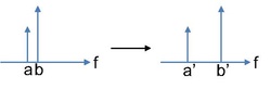
Now, we desire to explore the case of multiple frequencies, instead of a single frequency. The adjacent frequencies can be separated by the scaling c and modulation b properties. Namely, by randomly choosing the parameters of c and b, the distribution of all frequencies can be almost a uniform distribution. The figure Spread all frequencies reveals by randomly binning frequencies, we can utilize the single frequency recovery to seek the main components.
where c is scaling property and b is modulation property.
By randomly choosing c and b, the whole spectrum can be looked like uniform distribution. Then, taking them into filter banks can separate all frequencies, including Gaussians,[4] indicator functions,[5][6] spike trains,[7][8][9][10] and Dolph-Chebyshev filters.[11] Each bank only contains a single frequency.
The prototypical SFT
Generally, all SFT follows the three stages[1]
Identifying frequencies
By randomly bining frequencies, all components can be separated. Then, taking them into filter banks, so each band only contains a single frequency. It is convenient to use the methods we mentioned to recover this signal frequency.
Estimating coefficients
After identifying frequencies, we will have many frequency components. We can use Fourier transform to estimate their coefficients.
Repeating
Finally, repeating these two stages can we extract the most important components from the original signal.
Sparse Fourier transform in the discrete setting
In 2012, Hassanieh, Indyk, Katabi, and Price [11] proposed an algorithm that takes samples and runs in the same running time.
Sparse Fourier transform in the high dimensional setting
In 2014, Indyk and Kapralov [12] proposed an algorithm that takes samples and runs in nearly linear time in . In 2016, Kapralov [13] proposed an algorithm that uses sublinear samples and sublinear decoding time . In 2019, Nakos, Song, and Wang [14] introduced a new algorithm which uses nearly optimal samples and requires nearly linear time decoding time. A dimension-incremental algorithm was proposed by Potts, Volkmer [15] based on sampling along rank-1 lattices.
Sparse Fourier transform in the continuous setting
There are several works about generalizing the discrete setting into the continuous setting.[16][17]
Implementations
There are several works based on MIT, MSU, ETH and Universtity of Technology Chemnitz [TUC]. Also, they are free online.
Further reading
Hassanieh, Haitham (2018). The Sparse Fourier Transform: Theory and Practice. Association for Computing Machinery and Morgan & Claypool. ISBN 978-1-94748-707-9.
Price, Eric (2013). Sparse Recovery and Fourier Sampling. MIT.
References
- ↑ 1.0 1.1 Gilbert, Anna C.; Indyk, Piotr; Iwen, Mark; Schmidt, Ludwig (2014). "Recent Developments in the Sparse Fourier Transform: A compressed Fourier transform for big data". IEEE Signal Processing Magazine 31 (5): 91–100. doi:10.1109/MSP.2014.2329131. Bibcode: 2014ISPM...31...91G. https://dspace.mit.edu/bitstream/1721.1/113828/1/Recent%20developments.pdf.
- ↑ Cipra, Barry A. (2000). The best of the 20th century: Editors name top 10 algorithms. SIAM news 33.4.
- ↑ Iwen, M. A. (2010-01-05). "Combinatorial Sublinear-Time Fourier Algorithms". Foundations of Computational Mathematics 10 (3): 303–338. doi:10.1007/s10208-009-9057-1.
- ↑ Haitham Hassanieh; Piotr Indyk; Dina Katabi; Eric Price (2012). Simple and Practical Algorithm for Sparse Fourier Transform. pp. 1183–1194. doi:10.1137/1.9781611973099.93. ISBN 978-1-61197-210-8.
- ↑ A. C. Gilbert (2002). "Near-optimal sparse fourier representations via sampling". Proceedings of the thiry-fourth annual ACM symposium on Theory of computing. S. Guha, P. Indyk, S. Muthukrishnan, M. Strauss. pp. 152–161. doi:10.1145/509907.509933. ISBN 1581134959.
- ↑ A. C. Gilbert; S. Muthukrishnan; M. Strauss (21 September 2005). "Improved time bounds for near-optimal sparse Fourier representations". Wavelets XI. Proceedings of SPIE. 5914. pp. 59141A. doi:10.1117/12.615931. Bibcode: 2005SPIE.5914..398G.
- ↑ Ghazi, Badih; Hassanieh, Haitham; Indyk, Piotr; Katabi, Dina; Price, Eric; Lixin Shi (2013). "Sample-optimal average-case sparse Fourier Transform in two dimensions". 2013 51st Annual Allerton Conference on Communication, Control, and Computing (Allerton). pp. 1258–1265. doi:10.1109/Allerton.2013.6736670. ISBN 978-1-4799-3410-2.
- ↑ Iwen, M. A. (2010-01-05). "Combinatorial Sublinear-Time Fourier Algorithms". Foundations of Computational Mathematics 10 (3): 303–338. doi:10.1007/s10208-009-9057-1.
- ↑ Mark A.Iwen (2013-01-01). "Improved approximation guarantees for sublinear-time Fourier algorithms" (in en). Applied and Computational Harmonic Analysis 34 (1): 57–82. doi:10.1016/j.acha.2012.03.007. ISSN 1063-5203.
- ↑ Pawar, Sameer; Ramchandran, Kannan (2013). "Computing a k-sparse n-length Discrete Fourier Transform using at most 4k samples and O(k log k) complexity". 2013 IEEE International Symposium on Information Theory. pp. 464–468. doi:10.1109/ISIT.2013.6620269. ISBN 978-1-4799-0446-4.
- ↑ 11.0 11.1 Hassanieh, Haitham; Indyk, Piotr; Katabi, Dina; Price, Eric (2012). "Nearly optimal sparse fourier transform". Proceedings of the forty-fourth annual ACM symposium on Theory of computing. STOC'12. ACM. pp. 563–578. doi:10.1145/2213977.2214029. ISBN 9781450312455. https://dl.acm.org/citation.cfm?id=2214029.
- ↑ Indyk, Piotr; Kapralov, Michael (2014). "Sample-optimal Fourier sampling in any constant dimension". Annual Symposium on Foundations of Computer Science. FOCS'14: 514–523. https://archive.org/details/arxiv-1403.5804.
- ↑ Kapralov, Michael (2016). "Sparse fourier transform in any constant dimension with nearly-optimal sample complexity in sublinear time". Proceedings of the forty-eighth annual ACM symposium on Theory of Computing. STOC'16. pp. 264–277. doi:10.1145/2897518.2897650. ISBN 9781450341325. https://archive.org/details/arxiv-1604.00845.
- ↑ Nakos, Vasileios; Song, Zhao; Wang, Zhengyu (2019). "(Nearly) Sample-Optimal Sparse Fourier Transform in Any Dimension; RIPless and Filterless". Annual Symposium on Foundations of Computer Science. FOCS'19.
- ↑ Potts, Daniel; Volkmer, Toni (2016). "Sparse high-dimensional FFT based on rank-1 lattice sampling". Applied and Computational Harmonic Analysis 41 (3): 713–748. doi:10.1016/j.acha.2015.05.002.
- ↑ Price, Eric; Song, Zhao (2015). "A Robust Sparse Fourier Transform in the Continuous Setting". Annual Symposium on Foundations of Computer Science. FOCS'15: 583–600.
- ↑ Chen, Xue; Kane, Daniel M.; Price, Eric; Song, Zhao (2016). "Fourier-Sparse Interpolation without a Frequency Gap". Annual Symposium on Foundations of Computer Science. FOCS'16: 741–750. https://archive.org/details/arxiv-1609.01361.
 |  |
