Struve function

Graph of [math]\displaystyle{ \mathrm{H}_n(x) }[/math] for [math]\displaystyle{ n\in [0,1,2,3,4,5] }[/math]

In mathematics, the Struve functions H_α(x), are solutions y(x) of the non-homogeneous Bessel's differential equation:

[math]\displaystyle{ x^2 \frac{d^2 y}{dx^2} + x \frac{dy}{dx} + \left (x^2 - \alpha^2 \right )y = \frac{4\left (\frac{x}{2}\right)^{\alpha+1}}{\sqrt{\pi}\Gamma \left (\alpha+\frac{1}{2} \right )} }[/math]

introduced by Hermann Struve (1882). The complex number α is the order of the Struve function, and is often an integer.

And further defined its second-kind version [math]\displaystyle{ \mathbf{K}_\alpha(x) }[/math] as [math]\displaystyle{ \mathbf{K}_\alpha(x)=\mathbf{H}_\alpha(x)-Y_\alpha(x) }[/math].

The modified Struve functions L_α(x) are equal to −ie^{−iαπ / 2}H_α(ix), are solutions y(x) of the non-homogeneous Bessel's differential equation:

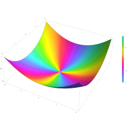
Plot of the Struve function H n(z) with n=2 in the complex plane from -2-2i to 2+2i with colors created with Mathematica 13.1 function ComplexPlot3D

[math]\displaystyle{ x^2 \frac{d^2 y}{dx^2} + x \frac{dy}{dx} - \left (x^2 + \alpha^2 \right )y = \frac{4\left (\frac{x}{2}\right)^{\alpha+1}}{\sqrt{\pi}\Gamma \left (\alpha+\frac{1}{2} \right )} }[/math]

And further defined its second-kind version [math]\displaystyle{ \mathbf{M}_\alpha(x) }[/math] as [math]\displaystyle{ \mathbf{M}_\alpha(x)=\mathbf{L}_\alpha(x)-I_\alpha(x) }[/math].

Definitions

Since this is a non-homogeneous equation, solutions can be constructed from a single particular solution by adding the solutions of the homogeneous problem. In this case, the homogeneous solutions are the Bessel functions, and the particular solution may be chosen as the corresponding Struve function.

Power series expansion

Struve functions, denoted as H_α(z) have the power series form

[math]\displaystyle{ \mathbf{H}_\alpha(z) = \sum_{m=0}^\infty \frac{(-1)^m}{\Gamma \left (m+\frac{3}{2} \right ) \Gamma \left (m+\alpha+\frac{3}{2} \right )} \left({\frac{z}{2}}\right)^{2m+\alpha+1}, }[/math]

where Γ(z) is the gamma function.

The modified Struve functions, denoted L_α(z), have the following power series form

[math]\displaystyle{ \mathbf{L}_\alpha(z) = \sum_{m=0}^\infty \frac{1}{\Gamma \left (m+\frac{3}{2} \right ) \Gamma \left (m+\alpha+\frac{3}{2} \right )} \left(\frac{z}{2}\right)^{2m+\alpha+1}. }[/math]

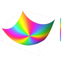
Plot of the modified Struve function L n(z) with n=2 in the complex plane from -2-2i to 2+2i with colors created with Mathematica 13.1 function ComplexPlot3D

Integral form

Another definition of the Struve function, for values of α satisfying Re(α) > − 1/2, is possible expressing in term of the Poisson's integral representation:

[math]\displaystyle{ \mathbf{H}_\alpha(x)=\frac{2\left(\frac{x}{2}\right)^\alpha}{\sqrt\pi\Gamma\left(\alpha+\frac{1}{2}\right)}\int_0^1(1-t^2)^{\alpha-\frac{1}{2}}\sin xt~dt=\frac{2\left(\frac{x}{2}\right)^\alpha}{\sqrt\pi\Gamma\left(\alpha+\frac{1}{2}\right)}\int_0^\frac{\pi}{2}\sin(x\cos\tau)\sin^{2\alpha}\tau~d\tau=\frac{2\left(\frac{x}{2}\right)^\alpha}{\sqrt\pi\Gamma\left(\alpha+\frac{1}{2}\right)}\int_0^\frac{\pi}{2}\sin(x\sin\tau)\cos^{2\alpha}\tau~d\tau }[/math]

[math]\displaystyle{ \mathbf{K}_\alpha(x)=\frac{2\left(\frac{x}{2}\right)^\alpha}{\sqrt\pi\Gamma\left(\alpha+\frac{1}{2}\right)}\int_0^\infty(1+t^2)^{\alpha-\frac{1}{2}}e^{-xt}~dt=\frac{2\left(\frac{x}{2}\right)^\alpha}{\sqrt\pi\Gamma\left(\alpha+\frac{1}{2}\right)}\int_0^\infty e^{-x\sinh\tau}\cosh^{2\alpha}\tau~d\tau }[/math]

[math]\displaystyle{ \mathbf{L}_\alpha(x)=\frac{2\left(\frac{x}{2}\right)^\alpha}{\sqrt\pi\Gamma\left(\alpha+\frac{1}{2}\right)}\int_0^1(1-t^2)^{\alpha-\frac{1}{2}}\sinh xt~dt=\frac{2\left(\frac{x}{2}\right)^\alpha}{\sqrt\pi\Gamma\left(\alpha+\frac{1}{2}\right)}\int_0^\frac{\pi}{2}\sinh(x\cos\tau)\sin^{2\alpha}\tau~d\tau=\frac{2\left(\frac{x}{2}\right)^\alpha}{\sqrt\pi\Gamma\left(\alpha+\frac{1}{2}\right)}\int_0^\frac{\pi}{2}\sinh(x\sin\tau)\cos^{2\alpha}\tau~d\tau }[/math]

[math]\displaystyle{ \mathbf{M}_\alpha(x)=-\frac{2\left(\frac{x}{2}\right)^\alpha}{\sqrt\pi\Gamma\left(\alpha+\frac{1}{2}\right)}\int_0^1(1-t^2)^{\alpha-\frac{1}{2}}e^{-xt}~dt=-\frac{2\left(\frac{x}{2}\right)^\alpha}{\sqrt\pi\Gamma\left(\alpha+\frac{1}{2}\right)}\int_0^\frac{\pi}{2}e^{-x\cos\tau}\sin^{2\alpha}\tau~d\tau=-\frac{2\left(\frac{x}{2}\right)^\alpha}{\sqrt\pi\Gamma\left(\alpha+\frac{1}{2}\right)}\int_0^\frac{\pi}{2}e^{-x\sin\tau}\cos^{2\alpha}\tau~d\tau }[/math]

Asymptotic forms

For small x, the power series expansion is given above.

For large x, one obtains:

[math]\displaystyle{ \mathbf{H}_\alpha(x) - Y_\alpha(x) = \frac{\left(\frac{x}{2}\right)^{\alpha-1}}{\sqrt{\pi} \Gamma \left (\alpha+\frac{1}{2} \right )} + O\left(\left (\tfrac{x}{2}\right)^{\alpha-3}\right), }[/math]

where Y_α(x) is the Neumann function.

Properties

The Struve functions satisfy the following recurrence relations:

[math]\displaystyle{ \begin{align} \mathbf{H}_{\alpha -1}(x) + \mathbf{H}_{\alpha+1}(x) &= \frac{2\alpha}{x} \mathbf{H}_\alpha (x) + \frac{\left (\frac{x}{2}\right)^{\alpha}}{\sqrt{\pi}\Gamma \left (\alpha + \frac{3}{2} \right )}, \\ \mathbf{H}_{\alpha -1}(x) - \mathbf{H}_{\alpha+1}(x) &= 2 \frac{d}{dx} \left (\mathbf{H}_\alpha(x) \right) - \frac{ \left( \frac{x}{2} \right)^\alpha}{\sqrt{\pi}\Gamma \left (\alpha + \frac{3}{2} \right )}. \end{align} }[/math]

Relation to other functions

Struve functions of integer order can be expressed in terms of Weber functions E_n and vice versa: if n is a non-negative integer then

[math]\displaystyle{ \begin{align} \mathbf{E}_n(z) &= \frac{1}{\pi} \sum_{k=0}^{\left \lfloor \frac{n-1}{2} \right \rfloor} \frac{\Gamma \left (k+ \frac{1}{2} \right) \left (\frac{z}{2} \right )^{n-2k-1}}{\Gamma \left (n- k + \frac{1}{2}\right )} -\mathbf{H}_n(z),\\ \mathbf{E}_{-n}(z) &= \frac{(-1)^{n+1}}{\pi}\sum_{k=0}^{\left \lfloor \frac{n-1}{2} \right \rfloor} \frac{\Gamma(n-k-\frac{1}{2}) \left (\frac{z}{2} \right )^{-n+2k+1}}{\Gamma \left (k+ \frac{3}{2} \right)}-\mathbf{H}_{-n}(z). \end{align} }[/math]

Struve functions of order n + 1/2 where n is an integer can be expressed in terms of elementary functions. In particular if n is a non-negative integer then

[math]\displaystyle{ \mathbf{H}_{-n-\frac{1}{2}} (z) = (-1)^n J_{n+\frac{1}{2}}(z), }[/math]

where the right hand side is a spherical Bessel function.

Struve functions (of any order) can be expressed in terms of the generalized hypergeometric function ₁F₂:

[math]\displaystyle{ \mathbf{H}_{\alpha}(z) = \frac{z^{\alpha+1}}{2^{\alpha}\sqrt{\pi} \Gamma \left (\alpha+\tfrac{3}{2} \right )} {}_1F_2 \left (1;\tfrac{3}{2}, \alpha+\tfrac{3}{2};-\tfrac{z^2}{4} \right ). }[/math]

Applications

The Struve and Weber functions were shown to have an application to beamforming in., and in describing the effect of confining interface on Brownian motion of colloidal particles at low Reynolds numbers.

References

• R. M. Aarts and Augustus J. E. M. Janssen (2003). "Approximation of the Struve function H₁ occurring in impedance calculations". J. Acoust. Soc. Am. 113 (5): 2635–2637. doi:10.1121/1.1564019. PMID 12765381. Bibcode: 2003ASAJ..113.2635A. 
• R. M. Aarts and Augustus J. E. M. Janssen (2016). "Efficient approximation of the Struve functions H_n occurring in the calculation of sound radiation quantities". J. Acoust. Soc. Am. 140 (6): 4154–4160. doi:10.1121/1.4968792. PMID 28040027. Bibcode: 2016ASAJ..140.4154A. https://research.tue.nl/nl/publications/efficient-approximation-of-the-struve-functions-hn-occurring-in-the-calculation-of-sound-radiation-quantaties(c68b8858-9c9d-4ff2-bf39-e888bb638527).html. 
• Abramowitz, Milton; Stegun, Irene Ann, eds (1983). "Chapter 12". Handbook of Mathematical Functions with Formulas, Graphs, and Mathematical Tables. Applied Mathematics Series. 55 (Ninth reprint with additional corrections of tenth original printing with corrections (December 1972); first ed.). Washington D.C.; New York: United States Department of Commerce, National Bureau of Standards; Dover Publications. pp. 496. LCCN 65-12253. ISBN 978-0-486-61272-0. http://www.math.sfu.ca/~cbm/aands/page_496.htm. 
• Hazewinkel, Michiel, ed. (2001), "S/s090700", Encyclopedia of Mathematics, Springer Science+Business Media B.V. / Kluwer Academic Publishers, ISBN 978-1-55608-010-4, https://www.encyclopediaofmath.org/index.php?title=S/s090700 
• Paris, R. B. (2010), "Struve function", in Olver, Frank W. J.; Lozier, Daniel M.; Boisvert, Ronald F. et al., NIST Handbook of Mathematical Functions, Cambridge University Press, ISBN 978-0-521-19225-5, http://dlmf.nist.gov/11 
• Struve, H. (1882). "Beitrag zur Theorie der Diffraction an Fernröhren". Annalen der Physik und Chemie 17 (13): 1008–1016. doi:10.1002/andp.18822531319. Bibcode: 1882AnP...253.1008S. https://zenodo.org/record/1423790. 

External links

• Struve functions at the Wolfram functions site.

References

- ↑ K. Buchanan, C. Flores, S. Wheeland, J. Jensen, D. Grayson and G. Huff, "Transmit beamforming for radar applications using circularly tapered random arrays," 2017 IEEE Radar Conference (RadarConf), 2017, pp. 0112-0117, doi: 10.1109/RADAR.2017.7944181
- ↑ B. U. Felderhof, "Effect of the wall on the velocity autocorrelation function and long-time tail of Brownian motion." The Journal of Physical Chemistry B 109.45, 2005, pp. 21406-21412