Super-resolution optical fluctuation imaging

Super-resolution optical fluctuation imaging (SOFI) is a post-processing method for the calculation of super-resolved images from recorded image time series that is based on the temporal correlations of independently fluctuating fluorescent emitters. SOFI has been developed for super-resolution of biological specimen that are labelled with independently fluctuating fluorescent emitters (organic dyes, fluorescent proteins). In comparison to other super-resolution microscopy techniques such as STORM or PALM that rely on single-molecule localization and hence only allow one active molecule per diffraction-limited area (DLA) and timepoint, SOFI does not necessitate a controlled photoswitching and/ or photoactivation as well as long imaging times. Nevertheless, it still requires fluorophores that are cycling through two distinguishable states, either real on-/off-states or states with different fluorescence intensities. In mathematical terms SOFI-imaging relies on the calculation of cumulants, for what two distinguishable ways exist. For one thing an image can be calculated via auto-cumulants that by definition only rely on the information of each pixel itself, and for another thing an improved method utilizes the information of different pixels via the calculation of cross-cumulants. Both methods can increase the final image resolution significantly although the cumulant calculation has its limitations. Actually SOFI is able to increase the resolution in all three dimensions.

Principle

Principle of the SOFI auto-cumulant calculation (A) Schematic depiction of a CCD-pixel grid containing several emitter-signals (B) Cut-out of two fluorophores with their signals convolved with the system's PSF, recorded in an image stack (C) The signals on every pixel are evaluated by cumulant calculation (a process that can be understood in terms of a correlation and integration)

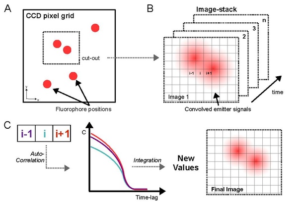
Likewise to other super-resolution methods SOFI is based on recording an image time series on a CCD- or CMOS camera. In contrary to other methods the recorded time series can be substantially shorter, since a precise localization of emitters is not required and therefore a larger quantity of activated fluorophores per diffraction-limited area is allowed. The pixel values of a SOFI-image of the n-th order are calculated from the values of the pixel time series in the form of a n-th order cumulant, whereas the final value assigned to a pixel can be imagined as the integral over a correlation function. The finally assigned pixel value intensities are a measure of the brightness and correlation of the fluorescence signal. Mathematically, the n-th order cumulant is related to the n-th order correlation function, but exhibits some advantages concerning the resulting resolution of the image. Since in SOFI several emitters per DLA are allowed, the photon count at each pixel results from the superposition of the signals of all activated nearby emitters. The cumulant calculation now filters the signal and leaves only highly correlated fluctuations. This provides a contrast enhancement and therefore a background reduction for good measure. As it is implied in the figure on the left the fluorescence source distribution:

[math]\displaystyle{ \sum_{k=1}^N \delta(\vec{r}-\vec{r}_{k})\cdot \varepsilon_k \cdot s_k(t) }[/math]

is convolved with the system's point spread function (PSF) U(r). Hence the fluorescence signal at time t and position [math]\displaystyle{ \vec{r} }[/math] is given by

[math]\displaystyle{ F(\vec{r},t)=\sum_{k=1}^N U(\vec{r}-\vec{r}_{k})\cdot \varepsilon_k \cdot s_k(t). }[/math]

Within the above equations N is the amount of emitters, located at the positions [math]\displaystyle{ \vec{r}_{k} }[/math] with a time-dependent molecular brightness [math]\displaystyle{ \varepsilon _{k}\cdot s_{k} }[/math] where [math]\displaystyle{ \varepsilon _{k} }[/math] is a variable for the constant molecular brightness and [math]\displaystyle{ s_k (t) }[/math] is a time-dependent fluctuation function. The molecular brightness is just the average fluorescence count-rate divided by the number of molecules within a specific region. For simplification it has to be assumed that the sample is in a stationary equilibrium and therefore the fluorescence signal can be expressed as a zero-mean fluctuation:

[math]\displaystyle{ \delta F(\vec{r},t)=F(\vec{r},t)-\langle F(\vec{r},t)\rangle_t }[/math]

where [math]\displaystyle{ \langle \cdots \rangle_t }[/math] denotes time-averaging. The auto-correlation here e.g. the second-order can then be described deductively as follows for a certain time-lag [math]\displaystyle{ \tau }[/math]:

[math]\displaystyle{ \delta F(\vec{r},t)=\langle \delta F(\vec{r},t+\tau )\cdot \delta F(\vec{r},t) \rangle_t }[/math]

From these equations it follows that the PSF of the optical system has to be taken to the power of the order of the correlation. Thus in a second-order correlation the PSF would be reduced along all dimensions by a factor of [math]\displaystyle{ \sqrt{2} }[/math]. As a result, the resolution of the SOFI-images increases according to this factor.

Cumulants versus correlations

Using only the simple correlation function for a reassignment of pixel values, would ascribe to the independency of fluctuations of the emitters in time in a way that no cross-correlation terms would contribute to the new pixel value. Calculations of higher-order correlation functions would suffer from lower-order correlations for what reason it is superior to calculate cumulants, since all lower-order correlation terms vanish.

Cumulant-calculation

Auto-cumulants

For computational reasons it is convenient to set all time-lags in higher-order cumulants to zero so that a general expression for the n-th order auto-cumulant can be found:

[math]\displaystyle{ AC_n(\vec{r},\tau_{1\ldots n-1} =0)=\sum_{k=1}^N U^n (\vec{r}-\vec{r}_k)\varepsilon^n_k w_k(0) }[/math]

[math]\displaystyle{ w_{k} }[/math] is a specific correlation based weighting function influenced by the order of the cumulant and mainly depending on the fluctuation properties of the emitters.

Albeit there is no fundamental limitation in calculating very high orders of cumulants and thereby shrinking the FWHM of the PSF there are practical limitations according to the weighting of the values assigned to the final image. Emitters with a higher molecular brightness will show a strong increase in terms of the pixel cumulant value assigned at higher-orders as well as this performance can be expected from a diverse appearance of fluctuations of different emitters. A wide intensity range of the resulting image can therefore be expected and as a result dim emitters can get masked by bright emitters in higher-order images:. The calculation of auto-cumulants can be realized in a very attractive way in a mathematical sense. The n-th order cumulant can be calculated with a basic recursion from moments

[math]\displaystyle{ K_n(\vec{r})=\mu_n (\vec{r})-\sum_{i=1}^{n-1} \begin{pmatrix}n-1\\i\end{pmatrix}K_{n-i}(\vec{r})\mu_i(\vec{r}) }[/math]

where K is a cumulant of the index's order, likewise [math]\displaystyle{ \mu }[/math] represents the moments. The term within the brackets indicates a binomial coefficient. This way of computation is straightforward in comparison with calculating cumulants with standard formulas. It allows for the calculation of cumulants with only little time of computing and is, as it is well implemented, even suitable for the calculation of high-order cumulants on large images.

Cross-cumulants

Principles of SOFI Cross-cumulant Calculation and Distance-factor: (A) 4th-order cross-cumulant calculation with "combinations with repetitions". (B) Distance-factor decay along the arrows.

In a more advanced approach cross-cumulants are calculated by taking the information of several pixels into account. Cross-cumulants can be described as follows:

[math]\displaystyle{ CC_n(\vec{r},\tau _{1\ldots n-1} =0)= \prod_{j\lt l}^{n}U\Bigg (\frac{\vec{r}_j-\vec{r}_l}{\sqrt{n}}\Bigg )\cdot \sum_{i=1}^N U^n \Bigg(\vec{r}_i-\frac{\sum_{k}^{n}\vec{r}_{k}}{n}\Bigg )\varepsilon^n_i w_i(0) }[/math]

j, l and k are indices for contributing pixels whereas i is the index for the current position. All other values and indices are used as before. The major difference in the comparison of this equation with the equation for the auto-cumulants is the appearance of a weighting-factor [math]\displaystyle{ U(r_{j}-r_{l}/\sqrt{n}) }[/math]. This weighting-factor (also termed distance-factor) is PSF-shaped and depends on the distance of the cross-correlated pixels in a sense that the contribution of each pixels decays along the distance in a PSF-shaped manner. In principle this means that the distance-factor is smaller for pixels that are further apart. The cross-cumulant approach can be used to create new, virtual pixels revealing true information about the labelled specimen by reducing the effective pixel size. These pixels carry more information than pixels that arise from simple interpolation.

In addition the cross-cumulant approach can be used to estimate the PSF of the optical system by making use of the intensity differences of the virtual pixels that is due to the "loss" in cross-correlation as aforementioned. Each virtual pixel can be re-weighted with the inverse of the distance-factor of the pixel leading to a restoration of the true cumulant value. At last the PSF can be used to create a resolution dependency of n for the nth-order cumulant by re-weighting the "optical transfer function" (OTF). This step can also be replaced by using the PSF for a deconvolution that is associated with less computational cost.

Cross-cumulant calculation requires the usage of a computational much more expensive formula that comprises the calculation of sums over partitions. This is of course owed to the combination of different pixels to assign a new value. Hence no fast recursive approach is usable at this point. For the calculation of cross-cumulants the following equation can be used:

[math]\displaystyle{ K_n \Bigg(\vec{r}=\frac{1}{n} \sum_{i=1}^n \vec{r_{i}}\Bigg)=\sum_P(-1)^{|P|-1}(|P|-1)!\prod_{p\in P}\Big\langle \prod_{i\in p} F(\vec{r})_{i}\Big\rangle_{t} }[/math]

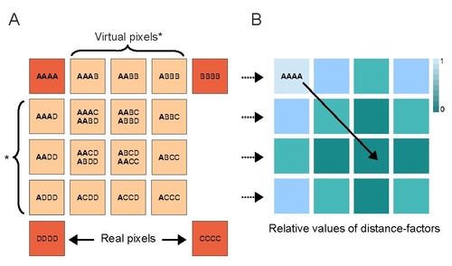
In this equation P denotes the amount of possible partitions, p denotes the different parts of each partition. In addition i is the index for the different pixel positions taken into account during the calculation what for F is just the image stack of the different contributing pixels. The cross-cumulant approach facilitates the generation of virtual pixels depending on the order of the cumulant as previously mentioned. These virtual pixels can be calculated in a particular pattern from the original pixels for a 4th-order cross-cumulant image, as it is depicted in the lower image, part A. The pattern itself arises simple from the calculation of all possible combinations of the original image pixels A, B, C and D. Here this was done by a scheme of "combinations with repetitions". Virtual pixels exhibit a loss in intensity that is due to the correlation itself. Part B of the second image depicts this general dependency of the virtual pixels on the cross-correlation. To restore meaningful pixel values the image is smoothed by a routine that defines a distance-factor for each pixel of the virtual pixel grid in a PSF-shaped manner and applies the inverse on all image pixels that are related to the same distance-factor.

References

- ↑ Eric Betzig, George H. Patterson, Rachid Sougrat, O. Wolf Lindwasser, Scott Olenych, Juan S. Bonifacino, Michael W. Davidson, Jennifer Lippincott-Schwartz, Harald F. Hess: Imaging Intracellular Fluorescent Proteins at Nanometer Resolution , Science, Vol. 313 no. 5793, 2006, pp. 1642–1645. doi:10.1126/science.1127344
- ↑ S. v.d.Linde, A. Löschberger, T. Klein, M. Heidbreder, S. Wolter, M. Heilemann, M. Sauer: Direct stochastical optical reconstruction microscopy with standard fluorescent probes , Nature Protocols, Vol. 6, 2011, pp. 991–1009. doi:10.1038/nprot.2011.336
- ↑ 3.0 3.1 3.2 3.3 3.4 T. Dertinger, R. Colyer, G. Iyer, S. Weiss, J. Enderlein: Fast, background-free, 3D super-resolution optical fluctuation imaging (SOFI) , PNAS, Vol. 106 no. 52, 2009, pp. 22287–22292. doi:10.1073/pnas.0907866106
- ↑ S. Geissbuehler, C. Dellagiacoma, T. Lasser: Comparison between SOFI and STORM , Biomedical Optics Express, Vol. 2 Issue 3, 2011, pp. 408–420. doi:10.1364/BOE.2.000408
- ↑ 5.0 5.1 5.2 5.3 5.4 5.5 T. Dertinger, R. Colyer, R. Vogel, J. Enderlein, S. Weiss: Achieving increased resolution and more pixels with Superresolution Optical Fluctuation Imaging (SOFI) , Optics Express, Vol. 18 Issue 18, 2010, pp. 18875–18885. doi:10.1364/OE.18.018875
- ↑ P. T. Smith: A Recursive Formulation of the Old Problem of Obtaining Moments from Cumulants and Vice Versa , The American Statistician, Vol. 49 Issue 2, 1995, pp. 217–218. doi:10.1080/00031305.1995.10476146
- ↑ 7.0 7.1 S. Geissbuehler, N.L. Bocchio, C. Dellagiacoma, C. Berclaz, M. Leutenegger, T. Lasser: Mapping molecular statistics with balanced super-resolution optical fluctuation imaging (bSOFI) , Optical Nanoscopy, Vol. 1, 2012, pp. 1–4. doi:10.1186/2192-2853-1-4
- ↑ J. M. Mendel: Tutorial on Higher-Order Statistics (Spectra) in Signal Processing and System Theory: Theoretical Results and Some Applications , Proceedings of the IEEE, Vol. 79 Issue 3, 1991, pp. 278–297. doi:10.1109/5.75086