Taylor–von Neumann–Sedov blast wave
Taylor–von Neumann–Sedov blast wave (or sometimes referred to as Sedov–von Neumann–Taylor blast wave) refers to a blast wave induced by a strong explosion. The blast wave was described by a self-similar solution independently by G. I. Taylor, John von Neumann and Leonid Sedov during World War II.[1][2]
History
G. I. Taylor was told by the British Ministry of Home Security that it might be possible to produce a bomb in which a very large amount of energy would be released by nuclear fission and asked to report the effect of such weapons. Taylor presented his results on June 27, 1941.[3] Exactly at the same time, in the United States , John von Neumann was working on the same problem and he presented his results on June 30, 1941.[4] It was said that Leonid Sedov was also working on the problem around the same time in the USSR, although Sedov never confirmed any exact dates.[5]
The complete solution was published first by Sedov in 1946.[6] von Neumann published his results in August 1947 in the Los Alamos scientific laboratory report on "Blast wave". https://apps.dtic.mil/dtic/tr/fulltext/u2/a384954.pdf., although that report was distributed only in 1958.[7] Taylor got clearance to publish his results in 1949 and he published his works in two papers in 1950.[8][9] In the second paper, Taylor calculated the energy of the atomic bomb used in the Trinity (nuclear test) using the similarity, just by looking at the series of blast wave photographs that had a length scale and time stamps, published by Julian E Mack in 1947.[10] This calculation of energy caused, in Taylor's own words, 'much embarrassment' (according to Grigory Barenblatt) in US government circles since the number was then still classified although the photographs published by Mack were not. Taylor's biographer George Batchelor writes This estimate of the yield of the first atom bomb explosion caused quite a stir... G.I. was mildly admonished by the US Army for publishing his deductions from their (unclassified) photographs.[11]
Mathematical description
Consider a strong explosion (such as nuclear bombs) that releases a large amount of energy [math]\displaystyle{ E }[/math] in a small volume during a short time interval. This will create a strong spherical shock wave propagating outwards from the explosion center. The self-similar solution tries to describe the flow when the shock wave has moved through a distance that is extremely large when compared to the size of the explosive. At these large distances, the information about the size and duration of the explosion will be forgotten; only the energy released [math]\displaystyle{ E }[/math] will have influence on how the shock wave evolves. To a very high degree of accuracy, then it can be assumed that the explosion occurred at a point (say the origin [math]\displaystyle{ r=0 }[/math]) instantaneously at time [math]\displaystyle{ t=0 }[/math].
The shock wave in the self-similar region is assumed to be still very strong such that the pressure behind the shock wave [math]\displaystyle{ p_1 }[/math] is very large in comparison with the pressure (atmospheric pressure) in front of the shock wave [math]\displaystyle{ p_0 }[/math], which can be neglected from the analysis. Although the pressure of the undisturbed gas is negligible, the density of the undisturbed gas [math]\displaystyle{ \rho_0 }[/math] cannot be neglected since the density jump across strong shock waves is finite as a direct consequence of Rankine–Hugoniot conditions. This approximation is equivalent to setting [math]\displaystyle{ p_0=0 }[/math] and the corresponding sound speed [math]\displaystyle{ c_0=0 }[/math], but keeping its density non zero, i.e., [math]\displaystyle{ \rho_0\neq 0 }[/math].[12]
The only parameters available at our disposal are the energy [math]\displaystyle{ E }[/math] and the undisturbed gas density [math]\displaystyle{ \rho_0 }[/math]. The properties behind the shock wave such as [math]\displaystyle{ p_1,\,\rho_1 }[/math] are derivable from those in front of the shock wave. The only non-dimensional combination available from [math]\displaystyle{ r,\,t,\,\rho_0 }[/math] and [math]\displaystyle{ E }[/math] is
- [math]\displaystyle{ r\left(\frac{\rho_0}{Et^2}\right)^{1/5} }[/math].
It is reasonable to assume that the evolution in [math]\displaystyle{ r }[/math] and [math]\displaystyle{ t }[/math] of the shock wave depends only on the above variable. This means that the shock wave location [math]\displaystyle{ r=R(t) }[/math] itself will correspond to a particular value, say [math]\displaystyle{ \beta }[/math], of this variable, i.e.,
- [math]\displaystyle{ R= \beta \left(\frac{Et^2}{\rho_0}\right)^{1/5}. }[/math]
The propagation velocity of the shock wave is
- [math]\displaystyle{ D=\frac{\mathrm{d}R}{\mathrm{d}t}=\frac{2R}{5t}=\frac{2\beta}{5}\left(\frac{E}{\rho_0t^3}\right)^{1/5} }[/math]
With the approximation described above, Rankine–Hugoniot conditions determines the gas velocity immediately behind the shock front [math]\displaystyle{ v_1 }[/math], [math]\displaystyle{ p_1 }[/math] and [math]\displaystyle{ \rho_1 }[/math] for an ideal gas as follows
- [math]\displaystyle{ v_1 = \frac{2}{\gamma+1}D, \quad p_1 = \frac{2}{\gamma+1}\rho_0 D^2, \quad \rho_1= \rho_0 \frac{\gamma+1}{\gamma-1} }[/math]
where [math]\displaystyle{ \gamma }[/math] is the specific heat ratio. Since [math]\displaystyle{ \rho_0 }[/math] is a constant, the density immediately behind the shock wave is not changing with time, whereas [math]\displaystyle{ v_1 }[/math] and [math]\displaystyle{ p_1 }[/math] decrease as [math]\displaystyle{ t^{-3/5} }[/math] and [math]\displaystyle{ t^{-6/5} }[/math], respectively.
Self-similar solution
The gas motion behind the shock wave is governed by Euler equations. For an ideal polytropic gas with spherical symmetry, the equations for the fluid variables such as radial velocity [math]\displaystyle{ v(r,t) }[/math], density [math]\displaystyle{ \rho(r,t) }[/math] and pressure [math]\displaystyle{ p(r,t) }[/math] are given by
- [math]\displaystyle{ \begin{align} \frac{\partial v}{\partial t} + v \frac{\partial v}{\partial r} &= - \frac{1}{\rho}\frac{\partial p}{\partial r},\\ \frac{\partial \rho}{\partial t} + \frac{\partial (\rho v)}{\partial r} &= - \frac{2\rho v}{r},\\ \left(\frac{\partial }{\partial t}+ v\frac{\partial }{\partial r}\right)\ln \frac{p}{\rho^\gamma} &=0. \end{align} }[/math]
At [math]\displaystyle{ r=R(t) }[/math], the solutions should approach the values given by the Rankine-Hugoniot conditions defined in the previous section.
The variable pressure can be replaced by the sound speed [math]\displaystyle{ c(r,t) }[/math] since pressure can be obtained from the formula [math]\displaystyle{ c^2=\gamma p/\rho }[/math]. The following non-dimensional self-similar variables are introduced,[13][14]
- [math]\displaystyle{ \xi = \frac{r}{R(t)}, \quad V(\xi) = \frac{5tv}{2r}, \quad G(\xi) = \frac{\rho}{\rho_0}, \quad Z(\xi) = \frac{25 t^2 c^2}{4r^2} }[/math].
The conditions at the shock front [math]\displaystyle{ \xi=1 }[/math] becomes
- [math]\displaystyle{ V(1) = \frac{2}{\gamma+1}, \quad G(1)=\frac{\gamma+1}{\gamma-1}, \quad Z(1) = \frac{2\gamma(\gamma-1)}{(\gamma+1)^2}. }[/math]
Substituting the self-similar variables into the governing equations will lead to three ordinary differential equations. Solving these differential equations analytically is laborious, as shown by Sedov in 1946 and von Neumann in 1947. G. I. Taylor integrated these equations numerically to obtain desired results.
The relation between [math]\displaystyle{ Z }[/math] and [math]\displaystyle{ V }[/math] can be deduced directly from energy conservation. Since the energy associated with the undisturbed gas is neglected by setting [math]\displaystyle{ p_0=0 }[/math], the total energy of the gas within the shock sphere must be equal to [math]\displaystyle{ E }[/math]. Due to self-similarity, it is clear that not only the total energy within a sphere of radius [math]\displaystyle{ \xi=1 }[/math] is constant, but also the total energy within a sphere of any radius [math]\displaystyle{ \xi\lt 1 }[/math] (in dimensional form, it says that total energy within a sphere of radius [math]\displaystyle{ r }[/math] that moves outwards with a velocity [math]\displaystyle{ v_n=2r/5t }[/math] must be constant). The amount of energy that leaves the sphere of radius [math]\displaystyle{ r }[/math] in time [math]\displaystyle{ dt }[/math] due to the gas velocity [math]\displaystyle{ v }[/math] is [math]\displaystyle{ 4\pi r^2\rho v(h+v^2/2)\mathrm{d}t }[/math], where [math]\displaystyle{ h }[/math] is the specific enthalpy of the gas. In that time, the radius of the sphere increases with the velocity [math]\displaystyle{ v_n }[/math] and the energy of the gas in this extra increased volume is [math]\displaystyle{ 4\pi r^2 \rho v_n(e+v^2/2)\mathrm{d}t }[/math], where [math]\displaystyle{ e }[/math] is the specific energy of the gas. Equating these expressions and substituting [math]\displaystyle{ e=c^2/\gamma(\gamma-1) }[/math] and [math]\displaystyle{ h=c^2/(\gamma-1) }[/math] that is valid for ideal polytropic gas leads to
- [math]\displaystyle{ Z = \frac{\gamma(\gamma-1)(1-V)V^2}{2(\gamma V-1)}. }[/math]
The continuity and energy equation reduce to
- [math]\displaystyle{ \begin{align} \frac{\mathrm{d} V }{\mathrm{d}\ln \xi} - (1-V) \frac{\mathrm{d}\ln G}{\mathrm{d}\ln\xi} &= - 3V\\ \frac{\mathrm{d}\ln Z}{\mathrm{d}\ln\xi} - (\gamma-1) \frac{\mathrm{d}\ln G}{\mathrm{d}\ln\xi} &= -\frac{5-2V}{1-V}. \end{align} }[/math]
Expressing [math]\displaystyle{ \mathrm{d}V/\mathrm{d}\ln\xi }[/math] and [math]\displaystyle{ \mathrm{d}\ln G/\mathrm{d}V }[/math] as a function of [math]\displaystyle{ V }[/math] only using the relation obtained earlier and integrating once yields the solution in implicit form,
- [math]\displaystyle{ \begin{align} \xi^5 &= \left[\frac{1}{2}(\gamma+1)V\right]^{-2} \left\{\frac{\gamma+1}{7-\gamma}[5-(3\gamma-1)V]\right\}^{\nu_1}\left[\frac{\gamma+1}{\gamma-1}(\gamma V-1)\right]^{\nu_2},\\ G &= \frac{\gamma+1}{\gamma-1}\left[\frac{\gamma+1}{\gamma-1}(\gamma V-1)\right]^{\nu_3}\left\{\frac{\gamma+1}{7-\gamma}[5-(3\gamma-1)V\right\}^{\nu_4}\left[\frac{\gamma+1}{\gamma-1}(1-V)\right]^{\nu_5} \end{align} }[/math]
where
- [math]\displaystyle{ \nu_1= -\frac{13\gamma^2-7\gamma+12}{(3\gamma-1)(2\gamma+1)},\quad \nu_2 = \frac{5(\gamma-1)}{2\gamma+1}, \quad \nu_3 = \frac{3}{2\gamma+1},\quad \nu_4 = -\frac{\nu_1}{2-\gamma}, \quad \nu_5 = - \frac{2}{2-\gamma}. }[/math]
The constant [math]\displaystyle{ \beta }[/math] that determines the shock location can be determined from the conservation of energy
- [math]\displaystyle{ E=\int_0^R\rho[v^2/2+c^2/\gamma(\gamma-1)]4\pi r^2\mathrm{d}r }[/math]
to obtain
- [math]\displaystyle{ \beta^5 \frac{16\pi}{25}\int_0^1 G[V^2/2+Z/\gamma(\gamma-1)]\xi^4\mathrm{d}\xi = 1. }[/math]
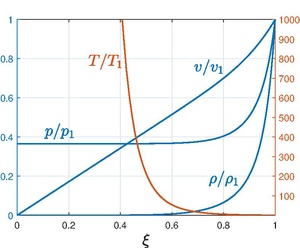
For air, [math]\displaystyle{ \gamma=7/5 }[/math] and [math]\displaystyle{ \beta=1.033 }[/math]. The solution for [math]\displaystyle{ \gamma=7/5 }[/math] is shown in the figure by graphing the curves of [math]\displaystyle{ \rho/\rho_1=G(\gamma-1)/(\gamma+1) }[/math], [math]\displaystyle{ v/v_1 = \xi V(\gamma+1)/2 }[/math], [math]\displaystyle{ p/p_1=\xi^2GZ(\gamma+1)/(2\gamma) }[/math] and [math]\displaystyle{ T/T_1=\xi^2Z(\gamma+1)^2/[2\gamma(\gamma-1)], }[/math] where [math]\displaystyle{ T }[/math] is the temperature.
Asymptotic behavior near the central region
The asymptotic behavior of the central region can be investigated by taking the limit [math]\displaystyle{ \xi\rightarrow 0 }[/math]. From the figure, it can be observed that the density falls to zero very rapidly behind the shock wave. The entire mass of the gas which was initially spread out uniformly in a sphere of radius [math]\displaystyle{ R }[/math] is now contained in a thin layer behind the shock wave, that is to say, all the mass is driven outwards by the acceleration imparted by the shock wave. Thus, most of the region is basically empty. The pressure ratio also drops rapidly to attain the constant value [math]\displaystyle{ p_c }[/math]. The temperature ratio follows from the ideal gas law; since density ratio decays to zero and the pressure ratio is constant, the temperature ratio must become infinite. The limiting form for the density is given as follows
- [math]\displaystyle{ \frac{\rho}{\rho_1} \sim \xi^{3/(\gamma-1)}, \quad \frac{p}{p_1}\rightarrow p_c, \quad \frac{T}{T_1} \sim \xi^{-3/(\gamma-1)} \quad \text{as} \quad \xi\rightarrow 0. }[/math]
Remember that the density [math]\displaystyle{ \rho_1 }[/math] is time-independent whereas [math]\displaystyle{ p_1\sim t^{-6/5} }[/math] which means that the actual pressure is in fact time dependent. It becomes clear if the above forms are rewritten in dimensional units,
- [math]\displaystyle{ \rho \sim r^{3/(\gamma-1)}t^{-6/5(\gamma-1)}, \quad p\rightarrow p_c t^{-6/5}, \quad T \sim r^{-3/(\gamma-1)}t^{(6/5)(2-\gamma)/(\gamma-1)} \quad \text{as} \quad r\rightarrow 0. }[/math]
The velocity ratio has the linear behavior in the central region,
- [math]\displaystyle{ \frac{v}{v_1} \sim \xi \quad \text{as} \quad \xi\rightarrow 0 }[/math]
whereas the behavior of the velocity itself is given by
- [math]\displaystyle{ v \sim r t^{1/5} \quad \text{as} \quad r\rightarrow 0. }[/math]
Final stage of the blast wave
As the shock wave evolves in time, its strength decreases. The self-similar solution described above breaks down when [math]\displaystyle{ p_1 }[/math] becomes comparable to [math]\displaystyle{ p_0 }[/math] (more precisely, when [math]\displaystyle{ p_1\sim [(\gamma+1)/(\gamma-1)]p_0 }[/math]). At this later stage of the evolution, [math]\displaystyle{ p_0 }[/math] (and consequently [math]\displaystyle{ c_0 }[/math]) cannot be neglected. This means that the evolution is not self-similar, because one can form a length scale [math]\displaystyle{ (E/p_0)^{1/3} }[/math] and a time scale [math]\displaystyle{ (E/p_0)^{1/3}/c_0 }[/math] to describe the problem. The governing equations are then integrated numerically, as was done by H. Goldstine and John von Neumann,[15] Brode,[16] and Okhotsimskii et al.[17]
Cylindrical line explosion
The analogous problem in cylindrical geometry corresponding to an axisymmetric blast wave can be solved analytically. This problem was solved independently by Leonid Sedov, A. Sakurai[18] and S. C. Lin.[19]
See also
References
- ↑ Bluman, G. W., & Cole, J. D. (2012). Similarity methods for differential equations (Vol. 13). Springer Science & Business Media.
- ↑ Barenblatt, G. I., Barenblatt, G. I., & Isaakovich, B. G. (1996). Scaling, self-similarity, and intermediate asymptotics: dimensional analysis and intermediate asymptotics (Vol. 14). Cambridge University Press.
- ↑ G. I. Taylor, British Report RC-210, June 27, 1941.
- ↑ John von Neumann, NDRC, Div. B, Report AM-9, June 30, 1941.
- ↑ Deakin, M. A. (2011). GI Taylor and the Trinity test. International Journal of Mathematical Education in Science and Technology, 42(8), 1069-1079.
- ↑ Sedov, L. I. (1946). Propagation of strong shock waves. Journal of Applied Mathematics and Mechanics, 10, 241-250.
- ↑ J. von Neumann, The point source solution, in Collected Works, Vol. 6, A.H. Taub, ed., Pergamon, New York, 1963, pp. 219–237.
- ↑ Taylor, G. I. (1950). The formation of a blast wave by a very intense explosion I. Theoretical discussion. Proceedings of the Royal Society of London. Series A. Mathematical and Physical Sciences, 201(1065), 159-174.
- ↑ Taylor, G. I. (1950). The formation of a blast wave by a very intense explosion.-II. The atomic explosion of 1945. Proceedings of the Royal Society of London. Series A. Mathematical and Physical Sciences, 201(1065), 175-186.
- ↑ Mack, J. E. (1946). Semi-popular motion-picture record of the Trinity explosion (Vol. 221). Technical Information Division, Oak Ridge Directed Operations.
- ↑ Batchelor, G. K., & Taylor, G. I. (1996). The life and legacy of GI Taylor. Cambridge University Press.
- ↑ Zelʹdovich, I. B., & Raĭzer, I. P. (1968). Physics of shock waves and high-temperature hydrodynamic phenomena (Vol. 1). Academic Press. Section 25. pp. 93-101.
- ↑ Landau, L. D., & Lifshitz, E. M. (1987). Fluid mechanics. Translated from the Russian by JB Sykes and WH Reid. Course of Theoretical Physics, 6. Section 106, pp. 403-407.
- ↑ Sedov, L. I. (1993). Similarity and dimensional methods in mechanics. CRC press.
- ↑ Goldstine, H. H., & Neumann, J. V. (1955). Blast wave calculation. Communications on Pure and Applied Mathematics, 8(2), 327-353.
- ↑ Brode, H. L. (1955). Numerical solutions of spherical blast waves. Journal of Applied physics, 26(6), 766-775.
- ↑ Okhotsimskii, D. E. E., Kondrasheva, I. L., Vlasova, Z. I., & Kazakova, R. K. (1957). Computation of point explosion taking into account counter-pressure. Trudy Matematicheskogo Instituta imeni VA Steklova, 50, 3-66.
- ↑ Sakurai, A. (1953). On the propagation and structure of the blast wave, I. Journal of the Physical Society of Japan, 8(5), 662-669.
- ↑ Lin, S. C. (1954). Cylindrical shock waves produced by instantaneous energy release. Journal of Applied Physics, 25(1), 54-57.
 |  |

