Physics:Two-dimensional correlation analysis

Two dimensional correlation analysis is a mathematical technique that is used to study changes in measured signals. As mostly spectroscopic signals are discussed, sometime also two dimensional correlation spectroscopy is used and refers to the same technique. In 2D correlation analysis, a sample is subjected to an external perturbation while all other parameters of the system are kept at the same value. This perturbation can be a systematic and controlled change in temperature, pressure, pH, chemical composition of the system, or even time after a catalyst was added to a chemical mixture. As a result of the controlled change (the perturbation), the system will undergo variations which are measured by a chemical or physical detection method. The measured signals or spectra will show systematic variations that are processed with 2D correlation analysis for interpretation.

When one considers spectra that consist of few bands, it is quite obvious to determine which bands are subject to a changing intensity. Such a changing intensity can be caused for example by chemical reactions. However, the interpretation of the measured signal becomes more tricky when spectra are complex and bands are heavily overlapping. Two dimensional correlation analysis allows one to determine at which positions in such a measured signal there is a systematic change in a peak, either continuous rising or drop in intensity. 2D correlation analysis results in two complementary signals, which referred to as the 2D synchronous and 2D asynchronous spectrum. These signals allow amongst others

1. to determine the events that are occurring at the same time (in phase) and those events that are occurring at different times (out of phase)
2. to determine the sequence of spectral changes
3. to identify various inter- and intramolecular interactions
4. band assignments of reacting groups
5. to detect correlations between spectra of different techniques, for example near infrared spectroscopy (NIR) and Raman spectroscopy

History

2D correlation analysis originated from 2D NMR spectroscopy. Isao Noda developed perturbation based 2D spectroscopy in the 1980s. This technique required sinusoidal perturbations to the chemical system under investigation. This specific type of the applied perturbation severely limited its possible applications. Following research done by several groups of scientists, perturbation based 2D spectroscopy could be developed to a more extended and generalized broader base. Since the development of generalized 2D correlation analysis in 1993 based on Fourier transformation of the data, 2D correlation analysis gained widespread use. Alternative techniques that were simpler to calculate, for example the disrelation spectrum, were also developed simultaneously. Because of its computational efficiency and simplicity, the Hilbert transform is nowadays used for the calculation of the 2D spectra. To date, 2D correlation analysis is used for the interpretation of many types of spectroscopic data (including XRF, UV/VIS spectroscopy, fluorescence, infrared, and Raman spectra), although its application is not limited to spectroscopy.

Properties of 2D correlation analysis

Demo dataset consisting of signals at specific intervals (1 out of 3 signals on a total of 15 signals is shown for clarity), peaks at 10 and 20 are rising in intensity whereas the peaks at 30 and 40 have a decreasing intensity

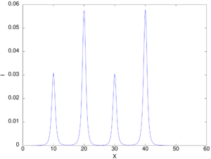
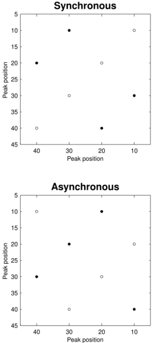
2D correlation analysis is frequently used for its main advantage: increasing the spectral resolution by spreading overlapping peaks over two dimensions and as a result simplification of the interpretation of one-dimensional spectra that are otherwise visually indistinguishable from each other. Further advantages are its ease of application and the possibility to make the distinction between band shifts and band overlap. Each type of spectral event, band shifting, overlapping bands of which the intensity changes in the opposite direction, band broadening, baseline change, etc. has a particular 2D pattern. See also the figure with the original dataset on the right and the corresponding 2D spectrum in the figure below.

Presence of 2D spectra

Schematic presence of a 2D correlation spectrum with peak positions represented by dots. Region A is the main diagonal containing autopeaks, off-diagonal regions B contain cross-peaks.

2D synchronous and asynchronous spectra are basically 3D-datasets and are generally represented by contour plots. X- and y-axes are identical to the x-axis of the original dataset, whereas the different contours represent the magnitude of correlation between the spectral intensities. The 2D synchronous spectrum is symmetric relative to the main diagonal. The main diagonal thus contains positive peaks. As the peaks at (x,y) in the 2D synchronous spectrum are a measure for the correlation between the intensity changes at x and y in the original data, these main diagonal peaks are also called autopeaks and the main diagonal signal is referred to as autocorrelation signal. The off-diagonal cross-peaks can be either positive or negative. On the other hand, the asynchronous spectrum is asymmetric and never has peaks on the main diagonal.

Generally contour plots of 2D spectra are oriented with rising axes from left to right and top to down. Other orientations are possible, but interpretation has to be adapted accordingly.

Calculation of 2D spectra

Suppose the original dataset D contains the n spectra in rows. The signals of the original dataset are generally preprocessed. The original spectra are compared to a reference spectrum. By subtracting a reference spectrum, often the average spectrum of the dataset, so called dynamic spectra are calculated which form the corresponding dynamic dataset E. The presence and interpretation may be dependent on the choice of reference spectrum. The equations below are valid for equally spaced measurements of the perturbation.

Calculation of the synchronous spectrum

A 2D synchronous spectrum expresses the similarity between spectral of the data in the original dataset. In generalized 2D correlation spectroscopy this is mathematically expressed as covariance (or correlation).

[math]\displaystyle{ \phi(\nu_1 , \nu_2) = \frac{1}{n-1} y^T(\nu_1) . y(\nu_2) }[/math]

where:

• Φ is the 2D synchronous spectrum
• ν₁ and ν₂ are two spectral channels
• y_ν is the vector composed of the signal intensities in E in column ν
• n the number of signals in the original dataset

Calculation of the asynchronous spectrum

Orthogonal spectra to the dynamic dataset E are obtained with the Hilbert-transform:

[math]\displaystyle{ \psi(\nu_1 , \nu_2) = \frac{1}{n-1} y^T(\nu_1) . N . y(\nu_2) }[/math]

where:

• Ψ is the 2D asynchronous spectrum
• ν₁ en ν₂ are two spectral channels
• y_ν is the vector composed of the signal intensities in E in column ν
• n the number of signals in the original dataset
• N the Noda-Hilbert transform matrix

The values of N, N_{j, k} are determined as follows:

• 0 if j = k
• [math]\displaystyle{ \frac{1}{\pi (k - j)} }[/math] if j ≠ k

where:

• j the row number
• k the column number

Interpretation

Interpretation of two-dimensional correlation spectra can be considered to consist of several stages.

Detection of peaks of which the intensity changes in the original dataset

Autocorrelation signal on the main diagonal of the synchronous 2D spectrum of the figure below (arbitrary axis units)

As real measurement signals contain a certain level of noise, the derived 2D spectra are influenced and degraded with substantial higher amounts of noise. Hence, interpretation begins with studying the autocorrelation spectrum on the main diagonal of the 2D synchronous spectrum. In the 2D synchronous main diagonal signal on the right 4 peaks are visible at 10, 20, 30, and 40 (see also the 4 corresponding positive autopeaks in the 2D synchronous spectrum on the right). This indicates that in the original dataset 4 peaks of changing intensity are present. The intensity of peaks on the autocorrelation spectrum are directly proportional to the relative importance of the intensity change in the original spectra. Hence, if an intense band is present at position x, it is very likely that a true intensity change is occurring and the peak is not due to noise.

Additional techniques help to filter the peaks that can be seen in the 2D synchronous and asynchronous spectra.

Determining the direction of intensity change

Example of a two-dimensional correlation spectrum. Open circles in this simplified view represent positive peaks, while discs represent negative peaks

It is not always possible to unequivocally determine the direction of intensity change, such as is for example the case for highly overlapping signals next to each other and of which the intensity changes in the opposite direction. This is where the off diagonal peaks in the synchronous 2D spectrum are used for:

1. if there is a positive cross-peak at (x, y) in the synchronous 2D spectrum, the intensity of the signals at x and y changes in the same direction
2. if there is a negative cross-peak at (x, y) in the synchronous 2D spectrum, the intensity of the signals at x and y changes in the opposite direction

As can be seen in the 2D synchronous spectrum on the right, the intensity changes of the peaks at 10 and 30 are related and the intensity of the peak at 10 and 30 changes in the opposite direction (negative cross-peak at (10,30)). The same is true for the peaks at 20 and 40.

Determining the sequence of events

Most importantly, with the sequential order rules, also referred to as Noda's rules, the sequence of the intensity changes can be determined. By carefully interpreting the signs of the 2D synchronous and asynchronous cross peaks with the following rules, the sequence of spectral events during the experiment can be determined:

1. if the intensities of the bands at x and y in the dataset are changing in the same direction, the synchronous 2D cross peak at (x,y) is positive
2. if the intensities of the bands at x and y in the dataset are changing in the opposite direction, the synchronous 2D cross peak at (x,y) is negative
3. if the change at x mainly precedes the change in the band at y, the asynchronous 2D cross peak at (x,y) is positive
4. if the change at x mainly follows the change in the band at y, the asynchronous 2D cross peak at (x,y) is negative
5. if the synchronous 2D cross peak at (x,y) is negative, the interpretation of rule 3 and 4 for the asynchronous 2D peak at (x,y) has to be reversed

where x and y are the positions on the x-xaxis of two bands in the original data that are subject to intensity changes.

Following the rules above. It can be derived that the changes at 10 and 30 occur simultaneously and the changes in intensity at 20 and 40 occur simultaneously as well. Because of the positive asynchronous cross-peak at (10, 20), the changes at 10 and 30 (predominantly) occur before the intensity changes at 20 and 40.

In some cases the Noda rules cannot be so readily implied, predominately when spectral features are not caused by simple intensity variations. This may occur when band shifts occur, or when a very erratic intensity variation is present in a given frequency range.

See also

• Correlation spectroscopy
• Fluorescence correlation spectroscopy
• Two-dimensional infrared spectroscopy

References

- ↑ Shin-Ichi Morita; Yasuhiro F. Miura; Michio Sugi; Yukihiro Ozaki (2005). "New correlation indices invariant to band shifts in generalized two-dimensional correlation infrared spectroscopy". Chemical Physics Letters 402 (251–257): 251–257. doi:10.1016/j.cplett.2004.12.038. Bibcode: 2005CPL...402..251M.
- ↑ Koichi Murayama; Boguslawa Czarnik-Matusewicz; Yuqing Wu; Roumiana Tsenkova; Yukihiro Ozaki (2000). "Comparison between conventional spectral analysis methods, chemometrics, and two-dimensional correlation spectroscopy in the analysis of near-infrared spectra of protein". Applied Spectroscopy 54 (7): 978–985. doi:10.1366/0003702001950715. Bibcode: 2000ApSpe..54..978M.
- ↑ 3.0 3.1 Shin-Ichi Morita; Yukihiro Ozaki (2002). "Pattern recognitions of band shifting, overlapping, and broadening using global phase description derived from generalized two-dimensional correlation spectroscopy". Applied Spectroscopy 56 (4): 502–508. doi:10.1366/0003702021954953. Bibcode: 2002ApSpe..56..502M.
- ↑ 4.0 4.1 4.2 4.3 Isao Noda; Yukihiro Ozaki (2004). Two-Dimensional Correlation Spectroscopy - Applications in Vibrational and Optical Spectroscopy. John Wiley & Sons Ltd.. ISBN 978-0-471-62391-5. https://books.google.com/books?id=5nE7_D_ppr8C.
- ↑ Boguslawa Czarnik-Matusewicz; Sylwia Pilorz; Lorna Ashton; Ewan W. Blanch (2006). "Potential pitfalls concerning visualization of the 2D results". Journal of Molecular Structure 799 (1–3): 253–258. doi:10.1016/j.molstruc.2006.03.064. Bibcode: 2006JMoSt.799..253C.
- ↑ Noda, Isao (1993). "Generalized Two-Dimensional Correlation Method Applicable to Infrared, Raman, and Other Types of Spectroscopy". Applied Spectroscopy 47 (9): 1329–1336. doi:10.1366/0003702934067694. Bibcode: 1993ApSpe..47.1329N.
- ↑ R. Buchet, Y. Wu; G. Lachenal; C. Raimbault; Yukihiro Ozaki (2006). "Selecting two-dimensional cross-correlation functions to enhance interpretation of near-infrared spectra of proteins". Applied Spectroscopy 55 (2): 155–162. doi:10.1366/0003702011951452. Bibcode: 2001ApSpe..55..155B.