Histogram matching
In image processing, histogram matching or histogram specification is the transformation of an image so that its histogram matches a specified histogram.[1] The well-known histogram equalization method is a special case in which the specified histogram is uniformly distributed.[2]
It is possible to use histogram matching to balance detector responses as a relative detector calibration technique. It can be used to normalize two images, when the images were acquired at the same local illumination (such as shadows) over the same location, but by different sensors, atmospheric conditions or global illumination.
Implementation
Consider a grayscale input image X. It has a probability density function pr(r), where r is a grayscale value, and pr(r) is the probability of that value. This probability can easily be computed from the histogram of the image by
[math]\displaystyle{ p_r (r_j )= {n_j \over n} }[/math]
Where nj is the frequency of the grayscale value rj, and n is the total number of pixels in the image.
Now consider a desired output probability density function pz(z). A transformation of pr(r) is needed to convert it to pz(z).
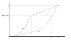
Each pdf (probability density function) can easily be mapped to its cumulative distribution function by
- [math]\displaystyle{ S(r_k )= \sum_{j=0}^k p_r(r_j),\qquad k = 0,1,2,3,\ldots,L-1 }[/math]
- [math]\displaystyle{ G(z_k )= \sum_{j=0}^k p_z(z_j),\qquad k = 0,1,2,3,\ldots,L-1 }[/math]
Where L is the total number of gray level (256 for a standard image).
The idea is to map each r value in X to the z value that has the same probability in the desired pdf. I.e. S(rj) = G(zi) or z = G−1(S(r)).[3]
Example
The following input grayscale image is to be changed to match the reference histogram.
The input image has the following histogram
It will be matched to this reference histogram to emphasize the lower gray levels.
After matching, the output image has the following histogramnone|thumb|1006x1006px|Histogram of output image after matchingAnd looks like thisFile:Output image.tif
Algorithm
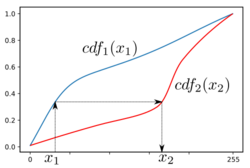
Given two images, the reference and the target images, we compute their histograms. Following, we calculate the cumulative distribution functions of the two images' histograms – [math]\displaystyle{ F_1()\, }[/math] for the reference image and [math]\displaystyle{ F_2()\, }[/math] for the target image. Then for each gray level [math]\displaystyle{ G_1\in[0,255] }[/math], we find the gray level [math]\displaystyle{ G_2\, }[/math] for which [math]\displaystyle{ F_1(G_1)=F_2(G_2)\, }[/math], and this is the result of histogram matching function: [math]\displaystyle{ M(G_1)=G_2\, }[/math]. Finally, we apply the function [math]\displaystyle{ M() }[/math] on each pixel of the reference image.
Exact histogram matching
In typical real-world applications, with 8-bit pixel values (discrete values in range [0, 255]), histogram matching can only approximate the specified histogram. All pixels of a particular value in the original image must be transformed to just one value in the output image.
Exact histogram matching is the problem of finding a transformation for a discrete image so that its histogram exactly matches the specified histogram.[4] Several techniques have been proposed for this. One simplistic approach converts the discrete-valued image into a continuous-valued image and adds small random values to each pixel so their values can be ranked without ties. However, this introduces noise to the output image.
Because of this there may be holes or open spots in the output matched histogram.
Multiple histogram matching
The histogram matching algorithm can be extended to find a monotonic mapping between two sets of histograms. Given two sets of histograms [math]\displaystyle{ P=\{p_i\}_{i=1}^k }[/math] and [math]\displaystyle{ Q = \{q_i \}_{i=1}^k }[/math], the optimal monotonic color mapping [math]\displaystyle{ M }[/math] is calculated to minimize the distance between the two sets simultaneously, namely [math]\displaystyle{ \operatorname{argmin}_M \sum_k d(M(p_k),q_k) }[/math] where [math]\displaystyle{ d(\cdot,\cdot) }[/math] is a distance metric between two histograms. The optimal solution is calculated using dynamic programming.[5]
See also
References
- ↑ Gonzalez, Rafael C.; Woods, Richard E. (2008). Digital Image Processing (3rd ed.). Prentice Hall. p. 128. ISBN 9780131687288.
- ↑ Gonzalez, R.C.; Fittes, B.A. (June 9–11, 1975). "Gray-level transformations for interactive image enhancement". 2nd Conference on Remotely Manned Systems: Technology and Applications. Los Angeles, California. pp. 17–19. https://ntrs.nasa.gov/archive/nasa/casi.ntrs.nasa.gov/19770022806.pdf#page=29.
- ↑ Gonzalez, Rafael (2017). Digital image processing 4th Edition. London: Pearson. pp. 94–103. ISBN 978-0133356724.
- ↑ Coltuc, Dinu; Bolon, Philippe; Chassery, Jean-Marc (May 2006). "Exact Histogram Specification". IEEE Transactions on Image Processing 15 (5): 1143–52. doi:10.1109/TIP.2005.864170. PMID 16671295. Bibcode: 2006ITIP...15.1143C. https://www.researchgate.net/publication/7109912.
- ↑ Shapira D.; Avidan S.; Hel-Or Y. (2013). "Multiple Histogram Matching". http://www.faculty.idc.ac.il/toky/Publications/Conference/hist_icip_13.pdf.
 |


