Second partial derivative test
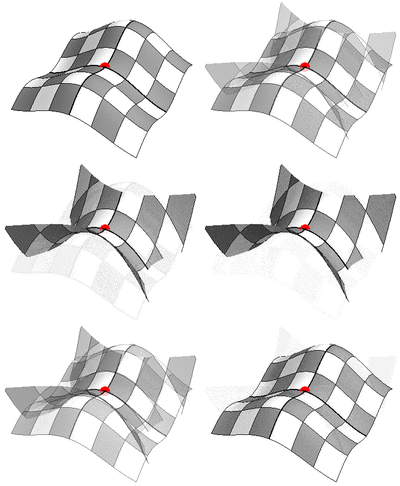
In mathematics, the second partial derivative test is a method in multivariable calculus used to determine if a critical point of a function is a local minimum, maximum or saddle point.
Functions of two variables
Suppose that f(x, y) is a differentiable real function of two variables whose second partial derivatives exist and are continuous. The Hessian matrix H of f is the 2 × 2 matrix of partial derivatives of f: [math]\displaystyle{ H(x,y) = \begin{bmatrix} f_{xx}(x,y) &f_{xy}(x,y)\\ f_{yx}(x,y) &f_{yy}(x,y) \end{bmatrix}. }[/math]
Define D(x, y) to be the determinant [math]\displaystyle{ D(x,y)=\det(H(x,y)) = f_{xx}(x,y)f_{yy}(x,y) - \left( f_{xy}(x,y) \right)^2 }[/math] of H. Finally, suppose that (a, b) is a critical point of f, that is, that fx(a, b) = fy(a, b) = 0. Then the second partial derivative test asserts the following:[1]
- If D(a, b) > 0 and fxx(a, b) > 0 then (a, b) is a local minimum of f.
- If D(a, b) > 0 and fxx(a, b) < 0 then (a, b) is a local maximum of f.
- If D(a, b) < 0 then (a, b) is a saddle point of f.
- If D(a, b) = 0 then the point (a, b) could be any of a minimum, maximum, or saddle point (that is, the test is inconclusive).
Sometimes other equivalent versions of the test are used. In cases 1 and 2, the requirement that fxx fyy − fxy2 is positive at (x, y) implies that fxx and fyy have the same sign there. Therefore, the second condition, that fxx be greater (or less) than zero, could equivalently be that fyy or tr(H) = fxx + fyy be greater (or less) than zero at that point.
A condition implicit in the statement of the test is that if [math]\displaystyle{ f_{xx} = 0 }[/math] or [math]\displaystyle{ f_{yy} = 0 }[/math], it must be the case that [math]\displaystyle{ D(a,b) \leq 0, }[/math] and therefore only cases 3 or 4 are possible.
Functions of many variables
For a function f of three or more variables, there is a generalization of the rule above. In this context, instead of examining the determinant of the Hessian matrix, one must look at the eigenvalues of the Hessian matrix at the critical point. The following test can be applied at any critical point a for which the Hessian matrix is invertible:
- If the Hessian is positive definite (equivalently, has all eigenvalues positive) at a, then f attains a local minimum at a.
- If the Hessian is negative definite (equivalently, has all eigenvalues negative) at a, then f attains a local maximum at a.
- If the Hessian has both positive and negative eigenvalues then a is a saddle point for f (and in fact this is true even if a is degenerate).
In those cases not listed above, the test is inconclusive.[2]
For functions of three or more variables, the determinant of the Hessian does not provide enough information to classify the critical point, because the number of jointly sufficient second-order conditions is equal to the number of variables, and the sign condition on the determinant of the Hessian is only one of the conditions. Note that in the one-variable case, the Hessian condition simply gives the usual second derivative test.
In the two variable case, [math]\displaystyle{ D(a, b) }[/math] and [math]\displaystyle{ f_{xx}(a,b) }[/math] are the principal minors of the Hessian. The first two conditions listed above on the signs of these minors are the conditions for the positive or negative definiteness of the Hessian. For the general case of an arbitrary number n of variables, there are n sign conditions on the n principal minors of the Hessian matrix that together are equivalent to positive or negative definiteness of the Hessian (Sylvester's criterion): for a local minimum, all the principal minors need to be positive, while for a local maximum, the minors with an odd number of rows and columns need to be negative and the minors with an even number of rows and columns need to be positive. See Hessian matrix for a discussion that generalizes these rules to the case of equality-constrained optimization.
Examples
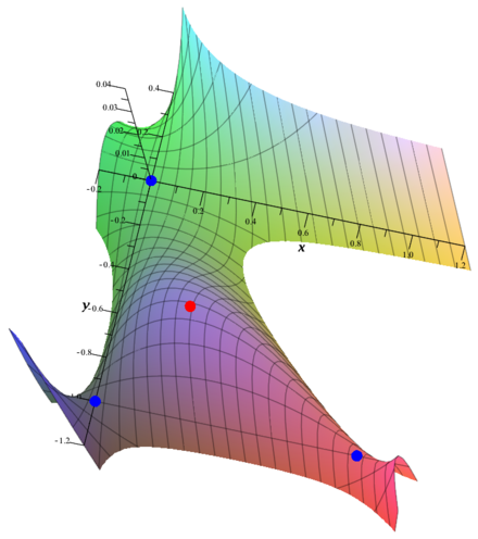
To find and classify the critical points of the function
- [math]\displaystyle{ z = f(x, y) = (x+y)(xy + xy^2) }[/math],
we first set the partial derivatives
- [math]\displaystyle{ \frac{\partial z}{\partial x} = y(2x +y)(y+1) }[/math] and [math]\displaystyle{ \frac{\partial z}{\partial y} = x \left( 3y^2 +2y(x+1) + x \right) }[/math]
equal to zero and solve the resulting equations simultaneously to find the four critical points
- [math]\displaystyle{ (0,0), (0, -1), (1,-1) }[/math] and [math]\displaystyle{ \left(\frac{3}{8}, -\frac{3}{4}\right) }[/math].
In order to classify the critical points, we examine the value of the determinant D(x, y) of the Hessian of f at each of the four critical points. We have
- [math]\displaystyle{ \begin{align} D(a, b) &= f_{xx}(a,b)f_{yy}(a,b) - \left( f_{xy}(a,b) \right)^2 \\ &= 2b(b+1) \cdot 2a(a + 3b + 1) - (2a + 2b + 4ab + 3b^2)^2. \end{align} }[/math]
Now we plug in all the different critical values we found to label them; we have
- [math]\displaystyle{ D(0, 0) = 0; ~~ D(0, -1) = -1; ~~ D(1, -1) = -1; ~~ D\left(\frac{3}{8}, -\frac{3}{4}\right) = \frac{27}{128}. }[/math]
Thus, the second partial derivative test indicates that f(x, y) has saddle points at (0, −1) and (1, −1) and has a local maximum at [math]\displaystyle{ \left(\frac{3}{8}, -\frac{3}{4}\right) }[/math] since [math]\displaystyle{ f_{xx} = -\frac{3}{8} \lt 0 }[/math]. At the remaining critical point (0, 0) the second derivative test is insufficient, and one must use higher order tests or other tools to determine the behavior of the function at this point. (In fact, one can show that f takes both positive and negative values in small neighborhoods around (0, 0) and so this point is a saddle point of f.)
Notes
- ↑ Stewart 2004, p. 803.
- ↑ Kurt Endl/Wolfgang Luh: Analysis II. Aula-Verlag 1972, 7th edition 1989, ISBN 3-89104-455-0, pp. 248-258 (German)
References
- James Stewart (2005). Multivariable Calculus: Concepts & Contexts. Brooks/Cole. ISBN 0-534-41004-9.
External links
- Relative Minimums and Maximums - Paul's Online Math Notes - Calc III Notes (Lamar University)
- Weisstein, Eric W.. "Second Derivative Test". http://mathworld.wolfram.com/SecondDerivativeTest.html.
 |


