Physics:Stress triaxiality

In continuum mechanics, stress triaxiality is the relative degree of hydrostatic stress in a given stress state. It is often used as a triaxiality factor, T.F, which is the ratio of the hydrostatic stress, ${\sigma }_m$, to the Von Mises equivalent stress, ${\sigma }_{eq}$. $\text{Missing argument for sqrt}$

Stress triaxiality has important applications in fracture mechanics and can often be used to predict the type of fracture (i.e. ductile or brittle) within the region defined by that stress state. A higher stress triaxiality corresponds to a stress state which is primarily hydrostatic rather than deviatoric. High stress triaxiality (> 2–3) promotes brittle cleavage fracture as well as dimple formation within an otherwise ductile fracture. Low stress triaxiality corresponds with shear slip and therefore larger ductility, as well as typically resulting in greater toughness. Ductile crack propagation is also influenced by stress triaxiality, with lower values producing steeper crack resistance curves. Several failure models such as the Johnson-Cook (J-C) fracture criterion (often used for high strain rate behavior), Rice-Tracey model, and J-Q large scale yielding model incorporate stress triaxiality.

History

In 1959 Davies and Connelly introduced so called triaxiality factor, defined as the ratio of Cauchy stress first principal invariant divided by effective stress ${\eta }_{DC}\equiv 3{\sigma }_m/{\sigma }_{ef}=I_1/\sqrt{3J_2}$, cf. formula (35) in Davies and Conelly (1959). The $I_1\equiv {\sigma }_I+{\sigma }_{II}+{\sigma }_{III}$ denotes first invariant of Cauchy stress tensor, ${\sigma }_I,{\sigma }_{II},{\sigma }_{III}$ denote principal values of Cauchy stress, ${\sigma }_m=\frac{1}{3}{I}_1$ denotes mean stress, $J_2\equiv \frac{1}{2}{s}_{ij}{s}_{ij}=\frac{1}{2}({s_I}^2+{s_{II}}^2+{s_{III}}^2)$ is second invariant of Cauchy stress deviator, $s_I,s_{II},s_{III}$ denote principal values of Cauchy stress deviator, ${\sigma }_{ef}\equiv \sqrt{3J_2}$ denotes effective stress.

Davies and Conelly were motivated in this proposal by supposition, correct in view of their own and later research, that negative pressure (spherical tension) $-p\equiv {\sigma }_m$ called by them rather exotically triaxial tension, has a strong influence on the loss of ductility of metals, and the need to have some parameter to describe this effect.

Wierzbicki and collaborators adopted a slightly modified definition of triaxiality factor than the original one $\eta \equiv {\sigma }_m/{\sigma }_{ef}\in <-\mathrm{\infty },\mathrm{\infty }>$, $\eta ={\eta }_{DC}/3$, cf. e.g. Wierzbicki et al (2005).

The name triaxiality factor is rather unfortunate, inadequate, because in physical terms the triaxiality factor determines the calibrated ratio of pressure forces relative to shearing forces or the ratio of isotropic (spherical) part of stress tensor in relation to its anisotropic (deviatoric) part both expressed in terms of their moduli, $\eta =(\sqrt{2}/3)||{\mathit{\sigma }}^{sph}||/||\mathbf{s}||$; $||{\mathit{\sigma }}^{sph}||=\sqrt{3}{\sigma }_m$, $||\mathbf{s}||=\sqrt{2J_2}$.

The triaxiality factor does not discern triaxial stress states from states of lower dimension.

Ziółkowski proposed to use as a measure of pressure towards shearing forces another modification of the index $\eta$, not burdened with whatever strength effort hypothesis, in the form ${\eta }_i\equiv ||{\mathit{\sigma }}^{sph}||/||\mathbf{s}||\in <-\mathrm{\infty },\mathrm{\infty }>$, cf. formula (8.2) in Ziółkowski (2022). In the context of material testing a reasonable mnemonic name for ${\eta }_i$ could be, e.g. pressure index or pressure factor.

Stress Triaxiality factor in biaxial tests

The triaxiality factor $\eta$ gained considerable attention and popularity when Wierzbicki and his collaborators pointed out that not only pressure ($-{\sigma }_m$) but also Lode angle ${\theta }_L$ can considerably influence ductile fracture and other properties of metals, cf. e.g. Wierzbicki et al (2005).

The class of biaxial tests is defined by the condition that always one of the principal values of the stress tensor is equal to zero (${\sigma }_{III}=0$). In 2005 Wierzbicki and Xue found that in the class of biaxial tests a unique constraint relation exists between normalized principal third invariant of deviator and triaxiality factor in the form $\xi =-(27/2)\eta ({\eta }^2-1/3)$, cf. formula (23) in Wierzbicki et al (2005).

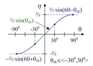
The normalized third invariant of stress deviator is defined as $\xi \equiv (27/2)(J_3/{{\sigma }_{ef}}^3)={\overline{J}}_3$, $\xi ={\overline{J}}_3\in <-1,1>$, where $J_3\equiv det(\mathbf{s})$ denotes third invariant of stress deviator .

In presentation of material testing results, the most frequently at present, it is used so called Lode angle ${\theta }_L$. The Lode angle is defined with the relation $cos(3{\theta }_L)\equiv {\overline{J}}_3,{\theta }_L\in <0,{60}^0>$. However, the Lode angle ${\theta }_L$ does not have clear (lucid) physical interpretation. From a mathematical standpoint, the Lode angle describes the angle between projection of Cauchy stress $\mathit{\sigma }$ on the octahedral plane and projection of the greatest principal stress ${\sigma }_I$ on the octahedral plane.

Ziółkowski proposed to use a skewness angle ${\theta }_{sk}$ defined with the following relation $\sin (3{\theta }_{sk})\equiv {\overline{J}}_3\in <-1,1>$, ${\theta }_{sk}\in <-{30}^0,{30}^0>$ for characterization of mode of shearing forces, cf. formula (4.2) in Ziółkowski (2022). The skewness angle ${\theta }_{sk}$ has several cogent and useful physical-statistical interpretations. It describes the departure of the actual Cauchy stress deviator $\mathbf{s}$ from the corresponding reference pure shear ${\mathbf{s}}_{ps}$, i.e., deviator with the same modulus as $\mathbf{s}$ $(||{\mathbf{s}}_{ps}||=||\mathbf{s}||)$ but with third invariant equal to zero $J_3({\mathbf{s}}_{ps})=det({\mathbf{s}}_{ps})=\frac{1}{3}tr({\mathbf{s}}_{ps})=0$.

Fig. Graphical illustration of the concepts of skewness angle ${\theta }_{sk}$ and Lode angle ${\theta }_L$, after Ziółkowski (2022).

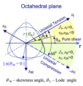
In micromechanical context the skewness angle can be understood as a macroscopic measure of the magnitude of internal entropy of the (macroscopic) Cauchy stress tensor. In this sense that its value determines degree of order of the population of micro pure shears (directional dipoles) generating the specific macroscopic stress state. The smaller is absolute values of skewness angle the smaller is internal entropy of Cauchy stress tensor.

The skewness angle enters as a parameter in a measure of anisotropy factor (degree) of stress tensor, which can be expressed with the formula ${\eta }_{ani}=\cos ({\theta }_{iso})\cdot \cos ({\theta }_{sk})$, cf. formula (4.5) in Ziółkowski (2022). The formula elucidates that the greater is internal order of pure shears population generating specific macroscopic stress state, i.e. the lower its entropy, the larger is anisotropy of the macroscopic stress tensor.

The ${\theta }_{iso}$ denotes isotropy angle defined with the formula $\sin ({\theta }_{iso})\equiv \mathbf{|}|{\mathit{\sigma }}^{sph}||/||\mathit{\sigma }||=\sqrt{3}{\sigma }_m/\sigma \in <-1,1>$, $\cos ({\theta }_{iso})\equiv ||\mathbf{s}||/||\mathit{\sigma }||=r/\sigma \in <0,1>$, $||\mathit{\sigma }||=\sqrt{3{{\sigma }_m}^2+2J_2}$, ${\theta }_{iso}\in <-{90}^0,{90}^0>$.

The isotropy angle enables extraction of the spherical (isotropic) part and deviatoric (anisotropic) part of the stress tensor in a very straightforward and convenient manner.

The measure of tensor anisotropy ${\eta }_{ani}$, introduced by Rychlewski (1985) and actually applicable to tensors of any degree, is defined with the formula ${\eta }_{ani}(\mathit{\sigma })\equiv d(\mathit{\sigma })/(2||\mathit{\sigma }||)$, ${\eta }_{ani}(\mathit{\sigma })\in <0,1>$.

The $d(\mathit{\sigma })$ denotes diameter of tensor orbit defined as follows, $d(\mathit{\sigma })=\underset{\mathbf{Q}\in \mathcal{R}}{max}\rho (\mathit{\sigma },\mathbf{Q}\mathit{\sigma }{\mathbf{Q}}^T)$, where $\rho$ denotes distance generated by the usual tensorial norm $\rho (\mathit{\alpha },\mathit{\beta })\equiv ||\mathit{\alpha }-\mathit{\beta }||$, $\mathbf{Q}\in \mathcal{R}$ is any second order proper orthogonal (rotation) tensor $\mathcal{R}=\{\mathbf{Q}\in {\mathcal{T}}^2;\mathbf{Q}{\mathbf{Q}}^T=\mathbf{1},det(\mathbf{Q})=+1\}$. The diameter of tensor orbit is simply a maximum distance between any two members in the orbit of a tensor $\mathit{\sigma }$.

A very simple (linear) connection exists between Lode angle and skewness angle ${\theta }_L={30}^0-{\theta }_{sk}$.

The Wierzbicki's constraint relation $\frac{1}{2}9\eta (1+\sqrt{3}\eta )(1-\sqrt{3}\eta )={\overline{J}}_3=\sin (3{\theta }_{sk})$, valid for biaxial stress states can be solved with respect to skewness angle to obtain the following explicit relations linking triaxiality factor and skewness angle, cf. Ziółkowski (2022).

$\begin{array}{rl}& \eta ({\theta }_{sk})=\frac{2}{3}\sin ({60}^0-{\theta }_{sk}),\eta \in <\frac{2}{3},\frac{1}{3}>,{\theta }_{sk}\in <-{30}^0,{30}^0>when{\sigma }_{III}=0\le {\sigma }_{II}\le {\sigma }_I,\\ & \eta ({\theta }_{sk})=\frac{2}{3}\sin ({\theta }_{sk}),\eta \in <-\frac{1}{3},\frac{1}{3}>,{\theta }_{sk}\in <-{30}^0,{30}^0>,when{\sigma }_{III}\le {\sigma }_{II}=0\le {\sigma }_I,\\ & \eta ({\theta }_{sk})=-\frac{2}{3}\sin ({60}^0+{\theta }_{sk}),\eta \in <-\frac{1}{3},-\frac{2}{3}>,{\theta }_{sk}\in <-{30}^0,{30}^0>,when{\sigma }_{III}\le {\sigma }_{II}\le {\sigma }_I=0;\\ & sign({\theta }_{sk})=sign({\overline{J}}_3),sign(\eta )=sign({\sigma }_m).\end{array}$

Fig. Graphical illustration of relation between triaxiality factor $\eta$ and skewness angle $\eta =\eta ({\theta }_{sk})$ valid for biaxial stress states, after Ziółkowski (2022).

The above relations $\eta ({\theta }_{sk})$ are three bijections (one to one relations) in three sharing edges but otherwise separate subdomains, which altogether make the entire two parameter domain (half-plane) of biaxial tests stress states.The explicit reverse relations ${\theta }_{sk}(\eta )$, easily obtainable from the above formulae, are very convenient for numerical computations, because they enable determination of the value of skewness (Lode) angle ${\theta }_{sk}$ (shearing mode of stress) only from the value of the triaxiality factor $\eta$ without the necessity to compute determinant of stress deviator, what delivers large computational savings. Selection of the correct subformula is very easy because it can be decided only upon the value of $\eta$ falling into a specific range of values. For example, when ${\eta }^{\ast }=0.51$, then it belongs to the range ${\eta }^{\ast }\in <\frac{1}{3},\frac{2}{3}>$; hence ${{\theta }_{sk}}^{\ast }={60}^0-{\sin }^{-1}(\frac{3}{2}{\eta }^{\ast })={10.1}^0$.

The relations $\eta ({\theta }_{sk})$ allowed for formulation and proof of the following important theorems and Corrollary, cf. Ziółkowski (2022).

Theorem I. The radial lines (rays) coming out from the origin $({\sigma }_I=0,{\sigma }_{II}=0)$ of the coordinates frame of the biaxial tests domain, i.e., half-plane $({\sigma }_{II}\le {\sigma }_I)$, are lines of constant values of triaxiality factor and at the same time, lines of constant values of skewness angle ${\theta }_{sk}=const,\eta =const$.

Theorem II. The relations ${\sigma }_m({\sigma }_{ef},{\theta }_{sk})$, ${\sigma }_{ef}({\sigma }_m,{\theta }_{sk})$, ${\theta }_{sk}({\sigma }_m,{\sigma }_{ef})$, valid for plane stress conditions, are bijections (one to one relations) in three sharing edges but otherwise separate subdomains of the whole domain of biaxial tests stress states, except on the line ${\sigma }_m=\frac{1}{3}({\sigma }_I+{\sigma }_{II})=0$, on which $\eta ={\theta }_{sk}=0$ for any value of ${\sigma }_{ef}=\sqrt{3}|{\sigma }_I|$.

Corollary. In the case of convex critical surface, with the aid of any type of biaxial (plane) stress test, for any fixed value of mean stress (pressure) ${\sigma }_m={{\sigma }_m}^{\ast }$, critical effective stress ${{\sigma }_{ef}}^{\ast }$ can be determined for only a single value of the skewness (Lode) angle ${{\theta }_{sk}}^{\ast }$, and thus corresponding to it single value of triaxiality factor $\eta ={\eta }^{\ast }$.

Fig. Graphical illustration of biaxial tests domain parameterization in terms of stress invariants $({\sigma }_m,{\sigma }_{ef},{\theta }_{sk})$. The $f({\mathit{\sigma }}^{cr})=0$ marks some hypothetical convex, critical surface of isotropic material, e.g., plastic yield. The 45⁰ slanted lines mark states with the same pressure, ellipsoids mark states with the same effective stress and radial lines from origin denote states with the same value of skewness (Lode) angle and simultaneously the same value of triaxiality factor, after Ziółkowski (2022).

In the case of convex critical surface, with the aid of any type of biaxial (plane) stress test, for any fixed value of skewness (Lode) angle ${\theta }_{sk}={{\theta }_{sk}}^{\ast }$, critical effective stresses ${{\sigma }_{ef}}^{\ast }$ can be determined for only three values of mean stress (pressure) ${\sigma }_m={{\sigma }_m}^{\ast }$, and thus three values of triaxiality factor $\eta ={\eta }^{\ast }$ corresponding to ${{\theta }_{sk}}^{\ast }$ in three subdomains.

The Corrollary indicates for limitations of the class of biaxial (plane) tests in experimental examination of the influence of skewness (Lode) angle and pressure on materials behavior submitted to multiaxial loadings. This is so, because upon executing only biaxial tests no adequate experimental data results can be collected to reliably separate the influence of mean stress and/or skewness angle on the possible variations of critical effective stresses. One value of skewness angle for any fixed pressure and/or three values of pressure for any fixed skewness angle deliver skimpy information for such purpose.

Triaxialy factor as convenient indicator showing transition from two-dimensional (plane) stress to full three-dimensional state of stress

Relations $\eta ({\theta }_{sk})$ valid for biaxial (plane) stress states show that in such a case, the values of the triaxiality factor must always remain in the range $\eta \in <-\frac{2}{3},\frac{2}{3}>$, while in the general case of three-dimensional multiaxial tests, the triaxiality factor can take any value from the range $\eta \in <-\mathrm{\infty },\mathrm{\infty }>$. In many experimental mechanics publications, in which results from biaxial tests are presented, values of triaxiality factor exceeding the two-third value can be encountered $\eta >\frac{2}{3},\eta <-\frac{2}{3},$ which may seem to be incorrect. However, experimental observation of the triaxiality factor greater than $\frac{2}{3}$ rather indicates that the biaxiality condition of the plane stress test was lost, and in the sample three-dimensional stress state started to exist, cf. Ziółkowski (2022).

References

1. Jump up to: 1.0 1.1 Fracture mechanics : twenty-fourth volume. Landes, J. D. (John D.), McCabe, Donald E., Boulet, Joseph Adrien Marie., ASTM Committee E-8 on Fatigue and Fracture., National Symposium on Fracture Mechanics (24th : 1992 : Gatlinburg, Tenn.). Philadelphia. pp. 89. ISBN 0-8031-1990-9. OCLC 32296916.
2. Hancock, J.W.; Mackenzie, A.C. (June 1976). "On the mechanisms of ductile failure in high-strength steels subjected to multi-axial stress-states" (in en). Journal of the Mechanics and Physics of Solids 24 (2-3): 147–160. doi:10.1016/0022-5096(76)90024-7. https://linkinghub.elsevier.com/retrieve/pii/0022509676900247.
3. Jump up to: 3.0 3.1 Soboyejo, W. O. (2003). "12.4.2 Cleavage Fracture". Mechanical properties of engineered materials. Marcel Dekker. ISBN 0-8247-8900-8. OCLC 300921090.
4. Lemaitre, Jean (1992) (in en). A Course on Damage Mechanics. Berlin, Heidelberg: Springer Berlin Heidelberg. pp. 45. doi:10.1007/978-3-662-02761-5. ISBN 978-3-662-02763-9. http://link.springer.com/10.1007/978-3-662-02761-5.
5. Jump up to: 5.0 5.1 Affonso, Luiz Octavio Amaral. (2013). Machinery Failure Analysis Handbook : Sustain Your Operations and Maximize Uptime.. Elsevier Science. pp. 33–42. ISBN 978-0-12-799982-1. OCLC 880756612.
6. Anderson, T. L. (Ted L.), 1957- (1995). Fracture mechanics : fundamentals and applications (2nd ed.). Boca Raton: CRC Press. pp. 87. ISBN 0-8493-4260-0. OCLC 31514487.
7. Dowling, N. E., Piascik, R. S., Newman, J. C. (1997). Fatigue and Fracture Mechanics: 27th Volume. United States: ASTM. (pp.75)
8. International Symposium on Ballistics (29th : 2016 : Edinburgh, Scotland), author. (2016). Proceedings 29th International Symposium on Ballistics : Edinburgh, Scotland, UK, 9-13 May 2016. pp. 1136–1137. ISBN 978-1-5231-1636-2. OCLC 1088722637.
9. Davies, E.A.; Connelly, F.M. (1959). "Stress distribution and plastic deformation in rotating cylinders of strain-hardening material". Journal of Applied Mechanics 26 (1): 25–30. doi:10.1115/1.4011918. Bibcode1959JAM....26...25D.
10. Jump up to: 10.0 10.1 10.2 Wierzbicki, T.; Bao, Y.; Lee, Y-W.; Bai, Y. (2005). "Calibration and evaluation of seven fracture models". International Journal of Mechanical Sciences 47 (4–5): 719–743. doi:10.1016/j.ijmecsci.2005.03.003.
11. Jump up to: 11.0 11.1 11.2 11.3 11.4 11.5 11.6 11.7 11.8 Ziółkowski, A.G. (2022). "Parametrization of Cauchy Stress Tensor Treated as Autonomous Object Using Isotropy Angle and Skewness Angle". Engineering Transactions 70 (2): 239–286. https://et.ippt.gov.pl/index.php/et/article/view/2210..
12. Rychlewski, J. (1985). "Zur Abschätzung der Anisotropie (To estimate the anisotropy)". Journal of Applied Mathematics and Mechanics 65 (6): 256–258. doi:10.1002/zamm.19850650617. https://engrxiv.org/preprint/view/1359/.