Prony's method
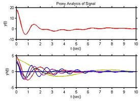
Prony analysis (Prony's method) was developed by Gaspard Riche de Prony in 1795. However, practical use of the method awaited the digital computer.[1] Similar to the Fourier transform, Prony's method extracts valuable information from a uniformly sampled signal and builds a series of damped complex exponentials or damped sinusoids. This allows the estimation of frequency, amplitude, phase and damping components of a signal.
The method
Let [math]\displaystyle{ f(t) }[/math] be a signal consisting of [math]\displaystyle{ N }[/math] evenly spaced samples. Prony's method fits a function
- [math]\displaystyle{ \hat{f}(t) = \sum_{i=1}^{N} A_i e^{\sigma_i t} \cos(\omega_i t + \phi_i) }[/math]
to the observed [math]\displaystyle{ f(t) }[/math]. After some manipulation utilizing Euler's formula, the following result is obtained, which allows more direct computation of terms:
- [math]\displaystyle{ \begin{align} \hat{f}(t) &= \sum_{i=1}^{N} A_i e^{\sigma_i t} \cos(\omega_i t + \phi_i) \\ &= \sum_{i=1}^{N} \frac{1}{2} A_i \left( e^{j\phi_i}e^{\lambda^+_i t} + e^{-j\phi_i}e^{\lambda^-_i t}\right), \end{align} }[/math]
where
- [math]\displaystyle{ \lambda^{\pm}_i = \sigma_i \pm j \omega_i }[/math] are the eigenvalues of the system,
- [math]\displaystyle{ \sigma_i = -\omega_{0,i} \xi_i }[/math] are the damping components,
- [math]\displaystyle{ \omega_i = \omega_{0,i} \sqrt{1-\xi_i^2} }[/math] are the angular-frequency components,
- [math]\displaystyle{ \phi_i }[/math] are the phase components,
- [math]\displaystyle{ A_i }[/math] are the amplitude components of the series,
- [math]\displaystyle{ j }[/math] is the imaginary unit ([math]\displaystyle{ j^2 = -1 }[/math]).
Representations
Prony's method is essentially a decomposition of a signal with [math]\displaystyle{ M }[/math] complex exponentials via the following process:
Regularly sample [math]\displaystyle{ \hat{f}(t) }[/math] so that the [math]\displaystyle{ n }[/math]-th of [math]\displaystyle{ N }[/math] samples may be written as
- [math]\displaystyle{ F_n = \hat{f}(\Delta_t n) = \sum_{m=1}^{M} \Beta_m e^{\lambda_m \Delta_t n}, \quad n=0,\dots,N-1. }[/math]
If [math]\displaystyle{ \hat{f}(t) }[/math] happens to consist of damped sinusoids, then there will be pairs of complex exponentials such that
- [math]\displaystyle{ \begin{align} \Beta_a &= \frac{1}{2} A_i e^{ \phi_i j}, \\ \Beta_b &= \frac{1}{2} A_i e^{-\phi_i j}, \\ \lambda_a &= \sigma_i + j \omega_i, \\ \lambda_b &= \sigma_i - j \omega_i, \end{align} }[/math]
where
- [math]\displaystyle{ \begin{align} \Beta_a e^{\lambda_a t} + \Beta_b e^{\lambda_b t} &= \frac{1}{2} A_i e^{\phi_i j} e^{(\sigma_i + j \omega_i) t} + \frac{1}{2}A_i e^{-\phi_i j} e^{(\sigma_i - j \omega_i) t} \\ &= A_i e^{\sigma_i t} \cos(\omega_i t + \phi_i). \end{align} }[/math]
Because the summation of complex exponentials is the homogeneous solution to a linear difference equation, the following difference equation will exist:
- [math]\displaystyle{ \hat{f}(\Delta_t n) = \sum_{m=1}^{M} \hat{f}[\Delta_t (n - m)] P_m, \quad n=M,\dots,N-1. }[/math]
The key to Prony's Method is that the coefficients in the difference equation are related to the following polynomial:
- [math]\displaystyle{ z^M - P_1 z^{M-1} - \dots - P_M = \prod_{m=1}^{M} \left(z - e^{\lambda_m}\right). }[/math]
These facts lead to the following three steps within Prony's method:
1) Construct and solve the matrix equation for the [math]\displaystyle{ P_m }[/math] values:
- [math]\displaystyle{ \begin{bmatrix} F_{M} \\ \vdots \\ F_{N-1} \end{bmatrix} = \begin{bmatrix} F_{M-1} & \dots & F_{0} \\ \vdots & \ddots & \vdots \\ F_{N-2} & \dots & F_{N-M-1} \end{bmatrix} \begin{bmatrix} P_1 \\ \vdots \\ P_M \end{bmatrix}. }[/math]
Note that if [math]\displaystyle{ N \ne 2M }[/math], a generalized matrix inverse may be needed to find the values [math]\displaystyle{ P_m }[/math].
2) After finding the [math]\displaystyle{ P_m }[/math] values, find the roots (numerically if necessary) of the polynomial
- [math]\displaystyle{ z^M - P_1 z^{M-1} - \dots - P_M. }[/math]
The [math]\displaystyle{ m }[/math]-th root of this polynomial will be equal to [math]\displaystyle{ e^{\lambda_m} }[/math].
3) With the [math]\displaystyle{ e^{\lambda_m} }[/math] values, the [math]\displaystyle{ F_n }[/math] values are part of a system of linear equations that may be used to solve for the [math]\displaystyle{ \Beta_m }[/math] values:
- [math]\displaystyle{ \begin{bmatrix} F_{k_1} \\ \vdots \\ F_{k_M} \end{bmatrix} = \begin{bmatrix} (e^{\lambda_1})^{k_1} & \dots & (e^{\lambda_M})^{k_1} \\ \vdots & \ddots & \vdots \\ (e^{\lambda_1})^{k_M} & \dots & (e^{\lambda_M})^{k_M} \end{bmatrix} \begin{bmatrix} \Beta_1 \\ \vdots \\ \Beta_M \end{bmatrix}, }[/math]
where [math]\displaystyle{ M }[/math] unique values [math]\displaystyle{ k_i }[/math] are used. It is possible to use a generalized matrix inverse if more than [math]\displaystyle{ M }[/math] samples are used.
Note that solving for [math]\displaystyle{ \lambda_m }[/math] will yield ambiguities, since only [math]\displaystyle{ e^{\lambda_m} }[/math] was solved for, and [math]\displaystyle{ e^{\lambda_m} = e^{\lambda_m \,+\, q 2 \pi j} }[/math] for an integer [math]\displaystyle{ q }[/math]. This leads to the same Nyquist sampling criteria that discrete Fourier transforms are subject to
- [math]\displaystyle{ \left|\operatorname{Im}(\lambda_m)\right| = \left|\omega_m\right| \lt \frac{\pi}{ \Delta_t}. }[/math]
See also
- Generalized pencil-of-function method
- Computation of Prony decomposition using Autoregression analysis
- Application of Prony decomposition in Time-frequency analysis
Notes
- ↑ Hauer, J. F.; Demeure, C. J.; Scharf, L. L. (1990). "Initial results in Prony analysis of power system response signals". IEEE Transactions on Power Systems 5: 80–89. doi:10.1109/59.49090.
References
- Carriere, R.; Moses, R. L. (1992). "High resolution radar target modeling using a modified Prony estimator". IEEE Transactions on Antennas and Propagation 40: 13–18. doi:10.1109/8.123348.
- Slyusar, V. I. (1998). "Interpretation of the Proni method for solving long-range problems". Radioelectronics and Communications Systems 41 (1): 35–39. http://slyusar.kiev.ua/en/IZV_1998_1.pdf.
 |


