ARGUS distribution

ARGUS

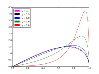
Probability density function c = 1.
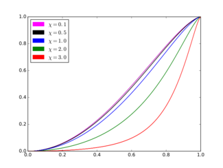
Cumulative distribution function c = 1.
Parameters	$c>0$ cut-off (real) $\chi >0$ curvature (real)
Support	$x\in (0,c)$
PDF	see text
CDF	see text
Mean	$\mu =c\sqrt{\pi /8}\frac{\chi e^{-\frac{{\chi }^2}{4}}{I}_1(\frac{{\chi }^2}{4})}{\mathrm{\Psi }(\chi )}$ where I1 is the Modified Bessel function of the first kind of order 1, and $\mathrm{\Psi }(x)$ is given in the text.
Mode	$\frac{c}{\sqrt{2}\chi }\sqrt{({\chi }^2-2)+\sqrt{{\chi }^4+4}}$
Variance	$c^2(1-\frac{3}{{\chi }^2}+\frac{\chi \varphi (\chi )}{\mathrm{\Psi }(\chi )})-{\mu }^2$

In physics, the ARGUS distribution, named after the particle physics experiment ARGUS, is the probability distribution of the reconstructed invariant mass of a decayed particle candidate in continuum background.

Definition

The probability density function (pdf) of the ARGUS distribution is:

$f(x;\chi ,c)=\frac{{\chi }^3}{\sqrt{2\pi }\mathrm{\Psi }(\chi )}\cdot \frac{x}{c^2}\sqrt{1-\frac{x^2}{c^2}}\exp \{-\frac{1}{2}{\chi }^2(1-\frac{x^2}{c^2}\left)\right\},$

for $0\le x<c$. Here $\chi$ and $c$ are parameters of the distribution and

$\mathrm{\Psi }(\chi )=\mathrm{\Phi }(\chi )-\chi \varphi (\chi )-\frac{1}{2},$

where $\mathrm{\Phi }(x)$ and $\varphi (x)$ are the cumulative distribution and probability density functions of the standard normal distribution, respectively.

Cumulative distribution function

The cumulative distribution function (cdf) of the ARGUS distribution is

$F(x)=1-\frac{\mathrm{\Psi }\left(\chi \sqrt{1-x^2/c^2}\right)}{\mathrm{\Psi }(\chi )}$.

Parameter estimation

Parameter c is assumed to be known (the kinematic limit of the invariant mass distribution), whereas χ can be estimated from the sample X₁, …, X_n using the maximum likelihood approach. The estimator is a function of sample second moment, and is given as a solution to the non-linear equation

$1-\frac{3}{{\chi }^2}+\frac{\chi \varphi (\chi )}{\mathrm{\Psi }(\chi )}=\frac{1}{n}\sum _{i=1}^n\frac{x_i^2}{c^2}$.

The solution exists and is unique, provided that the right-hand side is greater than 0.4; the resulting estimator $\hat{\chi }$ is consistent and asymptotically normal.

Generalized ARGUS distribution

Sometimes a more general form is used to describe a more peaking-like distribution:

$f(x)=\frac{2^{-p}{\chi }^{2(p+1)}}{\mathrm{\Gamma }(p+1)-\mathrm{\Gamma }(p+1,\frac{1}{2}{\chi }^2)}\cdot \frac{x}{c^2}{(1-\frac{x^2}{c^2})}^p\exp \{-\frac{1}{2}{\chi }^2(1-\frac{x^2}{c^2})\},0\le x\le c,c>0,\chi >0,p>-1$

$F(x)=\frac{\mathrm{\Gamma }(p+1,\frac{1}{2}{\chi }^2(1-\frac{x^2}{c^2}))-\mathrm{\Gamma }(p+1,\frac{1}{2}{\chi }^2)}{\mathrm{\Gamma }(p+1)-\mathrm{\Gamma }(p+1,\frac{1}{2}{\chi }^2)},0\le x\le c,c>0,\chi >0,p>-1$

where Γ(·) is the gamma function, and Γ(·,·) is the upper incomplete gamma function.

Here parameters c, χ, p represent the cutoff, curvature, and power respectively.

The mode is:

$\frac{c}{\sqrt{2}\chi }\sqrt{({\chi }^2-2p-1)+\sqrt{{\chi }^2({\chi }^2-4p+2)+(1+2p{)}^2}}$

The mean is:

$\mu =cp\sqrt{\pi }\frac{\mathrm{\Gamma }(p)}{\mathrm{\Gamma }(\frac{5}{2}+p)}\frac{{\chi }^{2p+2}}{2^{p+2}}\frac{M(p+1,\frac{5}{2}+p,-\frac{{\chi }^2}{2})}{\mathrm{\Gamma }(p+1)-\mathrm{\Gamma }(p+1,\frac{1}{2}{\chi }^2)}$

where M(·,·,·) is the Kummer's confluent hypergeometric function.

The variance is:

${\sigma }^2=c^2\frac{{\left(\frac{\chi }{2}\right)}^{p+1}{\chi }^{p+3}{e}^{-\frac{{\chi }^2}{2}}+({\chi }^2-2(p+1))\{\mathrm{\Gamma }(p+2)-\mathrm{\Gamma }(p+2,\frac{1}{2}{\chi }^2)\}}{{\chi }^2(p+1)(\mathrm{\Gamma }(p+1)-\mathrm{\Gamma }(p+1,\frac{1}{2}{\chi }^2))}-{\mu }^2$

p = 0.5 gives a regular ARGUS, listed above.

Further reading

• Albrecht, H. (1994). "Measurement of the polarization in the decay B → J/ψK*". Physics Letters B 340 (3): 217–220. doi:10.1016/0370-2693(94)01302-0. Bibcode: 1994PhLB..340..217A. 
• Pedlar, T.; Cronin-Hennessy, D.; Hietala, J.; Dobbs, S.; Metreveli, Z.; Seth, K.; Tomaradze, A.; Xiao, T. et al. (2011). "Observation of the h_c(1P) Using e⁺e⁻ Collisions above the DD Threshold". Physical Review Letters 107 (4): 041803. doi:10.1103/PhysRevLett.107.041803. PMID 21866994. Bibcode: 2011PhRvL.107d1803P. 
• Lees, J. P.; Poireau, V.; Prencipe, E.; Tisserand, V.; Garra Tico, J.; Grauges, E.; Martinelli, M.; Palano, A. et al. (2010). "Search for Charged Lepton Flavor Violation in Narrow Υ Decays". Physical Review Letters 104 (15): 151802. doi:10.1103/PhysRevLett.104.151802. PMID 20481982. Bibcode: 2010PhRvL.104o1802L.