Anscombe transform

Standard deviation of the transformed Poisson random variable as a function of the mean [math]\displaystyle{ m }[/math].

In statistics, the Anscombe transform, named after Francis Anscombe, is a variance-stabilizing transformation that transforms a random variable with a Poisson distribution into one with an approximately standard Gaussian distribution. The Anscombe transform is widely used in photon-limited imaging (astronomy, X-ray) where images naturally follow the Poisson law. The Anscombe transform is usually used to pre-process the data in order to make the standard deviation approximately constant. Then denoising algorithms designed for the framework of additive white Gaussian noise are used; the final estimate is then obtained by applying an inverse Anscombe transformation to the denoised data.

Anscombe transform animated. Here [math]\displaystyle{ \mu }[/math] is the mean of the Anscombe-transformed Poisson distribution, normalized by subtracting by [math]\displaystyle{ 2\sqrt{m + \tfrac{3}{8}} - \tfrac{1}{4 \, m^{1/2}} }[/math], and [math]\displaystyle{ \sigma }[/math] is its standard distribution (estimated empirically). We notice that [math]\displaystyle{ m^{3/2}\mu }[/math] and [math]\displaystyle{ m^2 (\sigma-1) }[/math] remains roughly in the range of [math]\displaystyle{ [0, 10] }[/math] over the period, giving empirical support for [math]\displaystyle{ \mu = O(m^{-3/2}), \sigma =1+ O(m^{-2}) }[/math]

Definition

For the Poisson distribution the mean [math]\displaystyle{ m }[/math] and variance [math]\displaystyle{ v }[/math] are not independent: [math]\displaystyle{ m = v }[/math]. The Anscombe transform

[math]\displaystyle{ A:x \mapsto 2 \sqrt{x + \tfrac{3}{8}} \, }[/math]

aims at transforming the data so that the variance is set approximately 1 for large enough mean; for mean zero, the variance is still zero.

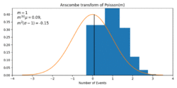
It transforms Poissonian data [math]\displaystyle{ x }[/math] (with mean [math]\displaystyle{ m }[/math]) to approximately Gaussian data of mean [math]\displaystyle{ 2\sqrt{m + \tfrac{3}{8}} - \tfrac{1}{4 \, m^{1/2}} + O\left(\tfrac{1}{m^{3/2}}\right) }[/math] and standard deviation [math]\displaystyle{ 1 + O\left(\tfrac{1}{m^2}\right) }[/math]. This approximation gets more accurate for larger [math]\displaystyle{ m }[/math], as can be also seen in the figure.

For a transformed variable of the form [math]\displaystyle{ 2 \sqrt{x + c} }[/math], the expression for the variance has an additional term [math]\displaystyle{ \frac{\tfrac{3}{8} -c}{m} }[/math]; it is reduced to zero at [math]\displaystyle{ c = \tfrac{3}{8} }[/math], which is exactly the reason why this value was picked.

Inversion

When the Anscombe transform is used in denoising (i.e. when the goal is to obtain from [math]\displaystyle{ x }[/math] an estimate of [math]\displaystyle{ m }[/math]), its inverse transform is also needed in order to return the variance-stabilized and denoised data [math]\displaystyle{ y }[/math] to the original range. Applying the algebraic inverse

[math]\displaystyle{ A^{-1}:y \mapsto \left( \frac{y}{2} \right)^2 - \frac{3}{8} }[/math]

usually introduces undesired bias to the estimate of the mean [math]\displaystyle{ m }[/math], because the forward square-root transform is not linear. Sometimes using the asymptotically unbiased inverse

[math]\displaystyle{ y \mapsto \left( \frac{y}{2} \right)^2 - \frac{1}{8} }[/math]

mitigates the issue of bias, but this is not the case in photon-limited imaging, for which the exact unbiased inverse given by the implicit mapping

[math]\displaystyle{ \operatorname{E} \left[ 2\sqrt{x+\tfrac{3}{8}} \mid m \right] = 2 \sum_{x=0}^{+\infty} \left( \sqrt{x+\tfrac{3}{8}} \cdot \frac{m^x e^{-m}}{x!} \right) \mapsto m }[/math]

should be used. A closed-form approximation of this exact unbiased inverse is

[math]\displaystyle{ y \mapsto \frac{1}{4} y^2 - \frac{1}{8} + \frac{1}{4} \sqrt{\frac{3}{2}} y^{-1} - \frac{11}{8} y^{-2} + \frac{5}{8} \sqrt{\frac{3}{2}} y^{-3}. }[/math]

Alternatives

There are many other possible variance-stabilizing transformations for the Poisson distribution. Bar-Lev and Enis report a family of such transformations which includes the Anscombe transform. Another member of the family is the Freeman-Tukey transformation

[math]\displaystyle{ A:x \mapsto \sqrt{x+1}+\sqrt{x}. \, }[/math]

A simplified transformation, obtained as the primitive of the reciprocal of the standard deviation of the data, is

[math]\displaystyle{ A:x \mapsto 2\sqrt{x} \, }[/math]

which, while it is not quite so good at stabilizing the variance, has the advantage of being more easily understood. Indeed, from the delta method,

[math]\displaystyle{ V[2\sqrt{x}] \approx \left(\frac{d (2\sqrt{m})}{d m} \right)^2 V[x] = \left(\frac{1}{\sqrt{m}} \right)^2 m = 1 }[/math].

Generalization

While the Anscombe transform is appropriate for pure Poisson data, in many applications the data presents also an additive Gaussian component. These cases are treated by a Generalized Anscombe transform and its asymptotically unbiased or exact unbiased inverses.

See also

• Variance-stabilizing transformation
• Box–Cox transformation

Further reading

• Starck, J.-L.; Murtagh, F. (2001), "Astronomical image and signal processing: looking at noise, information and scale", Signal Processing Magazine, IEEE 18 (2): 30–40, doi:10.1109/79.916319, Bibcode: 2001ISPM...18...30S

References

- ↑ 1.0 1.1 Anscombe, F. J. (1948), "The transformation of Poisson, binomial and negative-binomial data", Biometrika ([Oxford University Press, Biometrika Trust]) 35 (3–4): 246–254, doi:10.1093/biomet/35.3-4.246
- ↑ 2.0 2.1 Bar-Lev, S. K.; Enis, P. (1988), "On the classical choice of variance stabilizing transformations and an application for a Poisson variate", Biometrika 75 (4): 803–804, doi:10.1093/biomet/75.4.803
- ↑ Mäkitalo, M.; Foi, A. (2011), "Optimal inversion of the Anscombe transformation in low-count Poisson image denoising", IEEE Transactions on Image Processing 20 (1): 99–109, doi:10.1109/TIP.2010.2056693, PMID 20615809, Bibcode: 2011ITIP...20...99M
- ↑ Mäkitalo, M.; Foi, A. (2011), "A closed-form approximation of the exact unbiased inverse of the Anscombe variance-stabilizing transformation", IEEE Transactions on Image Processing 20 (9): 2697–2698, doi:10.1109/TIP.2011.2121085, PMID 21356615, Bibcode: 2011ITIP...20.2697M
- ↑ Freeman, M. F.; Tukey, J. W. (1950), "Transformations related to the angular and the square root", The Annals of Mathematical Statistics 21 (4): 607–611, doi:10.1214/aoms/1177729756
- ↑ Starck, J.L.; Murtagh, F.; Bijaoui, A. (1998). Image Processing and Data Analysis. Cambridge University Press. ISBN 9780521599146. https://archive.org/details/imageprocessingd0000star.
- ↑ Mäkitalo, M.; Foi, A. (2013), "Optimal inversion of the generalized Anscombe transformation for Poisson-Gaussian noise", IEEE Transactions on Image Processing 22 (1): 91–103, doi:10.1109/TIP.2012.2202675, PMID 22692910, Bibcode: 2013ITIP...22...91M