Astronomy:Regge–Wheeler–Zerilli equations
In general relativity, Regge–Wheeler–Zerilli equations are a pair of equations that describes gravitational perturbations of a Schwarzschild black hole, named after Tullio Regge, John Archibald Wheeler and Frank J. Zerilli.[1][2] The perturbations of a Schwarzchild metric is classified into two types, namely, axial and polar perturbations, a terminology introduced by Subrahmanyan Chandrasekhar. Axial perturbations induce frame dragging by imparting rotations to the black hole and change sign when azimuthal direction is reversed, whereas polar perturbations do not impart rotations and do not change sign under the reversal of azimuthal direction. The equation for axial perturbations is called Regge–Wheeler equation and the equation governing polar perturbations is called Zerilli equation.
The equations take the same form as the one-dimensional Schrödinger equation. The equations read as[3]
- [math]\displaystyle{ \left(\frac{d^2}{dr_*^2} + \sigma^2\right) Z^{\pm} = V^{\pm} Z^{\pm} }[/math]
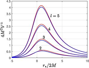
where [math]\displaystyle{ Z^+ }[/math] characterizes the polar perturbations and [math]\displaystyle{ Z^- }[/math] the axial perturbations. Here [math]\displaystyle{ r_*=r+2M\ln(r/2M-1) }[/math] is the tortoise coordinate (we set [math]\displaystyle{ G=c=1 }[/math]), [math]\displaystyle{ r }[/math] belongs to the Schwarzschild coordinates [math]\displaystyle{ (t,r,\theta,\varphi) }[/math], [math]\displaystyle{ 2M }[/math] is the Schwarzschild radius and [math]\displaystyle{ \sigma }[/math] representing the time-dependence of the perturbations appearing in the form [math]\displaystyle{ e^{i\sigma t} }[/math]. The Regge–Wheeler potential and Zerilli potential are respectively given by
- [math]\displaystyle{ V^{-}= \frac{2(r^2-2Mr)}{r^5}[(n+1)r-3M] }[/math]
- [math]\displaystyle{ V^{+}= \frac{2(r^2-2Mr)}{r^5(nr+3M)^2}[n^2(n+1)r^3+3Mn^2r^2+9M^2nr + 9M^3] }[/math]
where [math]\displaystyle{ 2n=(l-1)(l+2) }[/math] and [math]\displaystyle{ l=2,3,4,\dots }[/math] characterizes the eigenmode for the [math]\displaystyle{ \theta }[/math] coordinate. For gravitational perturbations, the modes [math]\displaystyle{ l=0,\,1 }[/math] are irrelevant because they do not evolve with time. Physically gravitational perturbations with [math]\displaystyle{ l=0 }[/math] (monopole) mode represents a change in the black hole mass, whereas the [math]\displaystyle{ l=1 }[/math] (dipole) mode corresponds to a shift in the location and value of the black hole's angular momentum. The shape of above potentials are exhibited in the figure.
Remember that in the tortoise coordinate, [math]\displaystyle{ r_* \rightarrow -\infty }[/math] denotes event horizon and [math]\displaystyle{ r_* \rightarrow \infty }[/math] is equivalent to [math]\displaystyle{ r\rightarrow \infty }[/math] i.e., to distances far away from the back hole. The potentials are short ranged as they decay faster than [math]\displaystyle{ 1/r_* }[/math]; as [math]\displaystyle{ r_*\rightarrow \infty }[/math], we have [math]\displaystyle{ V^{\pm}\rightarrow 2(n+1)/r^2 }[/math] and as [math]\displaystyle{ r_*\rightarrow -\infty }[/math], we have [math]\displaystyle{ V^{\pm}\sim e^{r_*/2M}. }[/math] Consequently, the asymptotic behaviour of the solutions for [math]\displaystyle{ r_*\rightarrow \pm\infty }[/math] is [math]\displaystyle{ e^{\pm i\sigma r_*}. }[/math]
Relations between the two problems
In 1975, Subrahmanyan Chandrasekhar and Steven Detweiler discovered a one-to-one mapping between the two equations, leading to a consequence that the spectrum corresponding to both potentials are identical.[4] The two potentials can also be written as
- [math]\displaystyle{ V^{\pm} = \pm 6M \frac{df}{dr_*} + (6Mf)^2 + 4n(n+1) f, \quad f = \frac{r^2-2Mr}{2r^3(nr+3M)}. }[/math]
The relations between [math]\displaystyle{ Z^+ }[/math] and [math]\displaystyle{ Z^- }[/math] are given by
- [math]\displaystyle{ [4n(n+1)\pm 12 i \sigma M] Z^{\pm} = \left[4n(n+1) + \frac{72M^2(r^2-2Mr)}{r^3(2nr+6M)}\right] Z^{\mp} \pm 12M \frac{dZ^{\mp}}{dr_*}. }[/math]
Reflection and transmission coefficients
Here [math]\displaystyle{ V^{\pm} }[/math] is always positive and the problem is one of reflection and transmission of waves incident from [math]\displaystyle{ r_*\rightarrow \infty }[/math] to [math]\displaystyle{ r_*\rightarrow -\infty }[/math]. The problem is essentially the same as that of a reflection and transmission problem by a potential barrier in quantum mechanics. Let the incident wave with unit amplitude be [math]\displaystyle{ e^{+i\sigma r_*} }[/math], then the asymptotic behaviours of the solution are given by
- [math]\displaystyle{ Z^{\pm} = e^{+i\sigma r_*} + R^{\pm} e^{-i\sigma r_*} \quad \text{as} \quad r_*\rightarrow +\infty }[/math]
- [math]\displaystyle{ Z^{\pm} = T^{\pm} e^{i\sigma r_*} \quad \text{as} \quad r_*\rightarrow -\infty }[/math]
where [math]\displaystyle{ R=R(\sigma) }[/math] and [math]\displaystyle{ T=T(\sigma) }[/math] are respectively are the reflection and transmission amplitudes. In the second equation, we have imposed the physical requirement that no waves emerge from the event horizon.
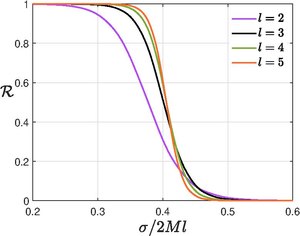
The reflection and transmission coefficients are thus defined as
- [math]\displaystyle{ \mathcal{R}^{\pm}=|R^{\pm}|^2, \quad \mathcal{T}^{\pm}=|T^{\pm}|^2 }[/math]
subjected to the condition [math]\displaystyle{ \mathcal{R}^{\pm}+ \mathcal{T}^{\pm}=1. }[/math] Because of the inherent connection between the two equations as outlined in the previous section, it turns out
- [math]\displaystyle{ T^+=T^-,\quad R^+ = e^{i\delta}R^-, \quad e^{i\delta}=\frac{4n(n+1)-12i\sigma M}{4n(n+1)+12 i\sigma M} }[/math]
and thus consequently, since [math]\displaystyle{ R^+ }[/math] and [math]\displaystyle{ R^- }[/math] differ only in their phases, we get
- [math]\displaystyle{ \mathcal{T}\equiv \mathcal{T}^{+}=\mathcal{T}^{-}, \quad \mathcal{R}\equiv\mathcal{R}^{+}=\mathcal{R}^{-}. }[/math]
Quasi-normal modes
Quasi-normal modes correspond to pure tones of the black hole. It describes for arbitrary, but small, perturbations such as an object falling into the black hole, accretion of matter surrounding it, last stage of slightly aspherical collapse etc. Perturbations are of damping type and thus corresponds to complex values of [math]\displaystyle{ \sigma }[/math]. The required boundary conditions are
- [math]\displaystyle{ Z^{\pm} = A^{\pm} e^{-i\sigma r_*} \quad \text{as} \quad r_*\rightarrow +\infty }[/math]
- [math]\displaystyle{ Z^{\pm} = e^{i\sigma r_*} \quad \text{as} \quad r_*\rightarrow -\infty }[/math]
indicating that we have purely outgoing waves with amplitude [math]\displaystyle{ A^{\pm} }[/math] and purely ingoing waves at the horizon.
The problem becomes an eigenvalue problem. Again because of the relation mentioned between the two problem, the spectrum of [math]\displaystyle{ Z^+ }[/math] and [math]\displaystyle{ Z^- }[/math] are identical and thus it enough to consider the spectrum of [math]\displaystyle{ Z^-. }[/math] The problem is simplified by introducing[4]
- [math]\displaystyle{ Z^-=\exp\left(i\int^{r_*} \phi \,dr_*\right). }[/math]
The nonlinear eigenvalue problem is given by
- [math]\displaystyle{ i \frac{d\phi}{dr_*} + \sigma^2 - \phi^2 - V^-=0, \quad \phi(-\infty)=+\sigma, \quad \phi(+\infty) =-\sigma. }[/math]
The solution is found to exist only for a discrete set of values of [math]\displaystyle{ \sigma. }[/math][5]
References
- ↑ Regge, T., & Wheeler, J. A. (1957). Stability of a Schwarzschild singularity. Physical Review, 108(4), 1063.
- ↑ Zerilli, F. J. (1970). Effective potential for even-parity Regge-Wheeler gravitational perturbation equations. Physical Review Letters, 24(13), 737.
- ↑ Chandrasekhar, S.(1983). The mathematical theory of black holes. Oxford university press.
- ↑ 4.0 4.1 Chandrasekhar, S., & Detweiler, S. (1975). The quasi-normal modes of the Schwarzschild black hole. Proceedings of the Royal Society of London. A. Mathematical and Physical Sciences, 344(1639), 441-452.
- ↑ Nollert, H. P. (1993). Quasinormal modes of Schwarzschild black holes: The determination of quasinormal frequencies with very large imaginary parts. Physical Review D, 47(12), 5253.
 |  |

