Bicubic interpolation

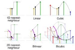
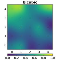
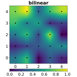
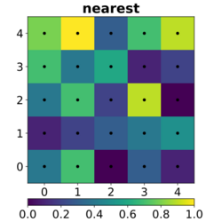
In mathematics, bicubic interpolation is an extension of cubic spline interpolation (a method of applying cubic interpolation to a data set) for interpolating data points on a two-dimensional regular grid. The interpolated surface (meaning the kernel shape, not the image) is smoother than corresponding surfaces obtained by bilinear interpolation or nearest-neighbor interpolation. Bicubic interpolation can be accomplished using either Lagrange polynomials, cubic splines, or cubic convolution algorithm.
In image processing, bicubic interpolation is often chosen over bilinear or nearest-neighbor interpolation in image resampling, when speed is not an issue. In contrast to bilinear interpolation, which only takes 4 pixels (2×2) into account, bicubic interpolation considers 16 pixels (4×4). Images resampled with bicubic interpolation can have different interpolation artifacts, depending on the b and c values chosen.
Computation


Suppose the function values and the derivatives , and are known at the four corners , , , and of the unit square. The interpolated surface can then be written as
The interpolation problem consists of determining the 16 coefficients . Matching with the function values yields four equations:
Likewise, eight equations for the derivatives in the and the directions:
And four equations for the mixed partial derivative:
The expressions above have used the following identities:
This procedure yields a surface on the unit square that is continuous and has continuous derivatives. Bicubic interpolation on an arbitrarily sized regular grid can then be accomplished by patching together such bicubic surfaces, ensuring that the derivatives match on the boundaries.
Grouping the unknown parameters in a vector and letting the above system of equations can be reformulated into a matrix for the linear equation .
Inverting the matrix gives the more useful linear equation , where which allows to be calculated quickly and easily.
There can be another concise matrix form for 16 coefficients: or where
Extension to rectilinear grids
Often, applications call for bicubic interpolation using data on a rectilinear grid, rather than the unit square. In this case, the identities for and become where is the spacing of the cell containing the point and similar for . In this case, the most practical approach to computing the coefficients is to let then to solve with as before. Next, the normalized interpolating variables are computed as where and are the and coordinates of the grid points surrounding the point . Then, the interpolating surface becomes
Finding derivatives from function values
If the derivatives are unknown, they are typically approximated from the function values at points neighbouring the corners of the unit square, e.g. using finite differences.
To find either of the single derivatives, or , using that method, find the slope between the two surrounding points in the appropriate axis. For example, to calculate for one of the points, find for the points to the left and right of the target point and calculate the slope of the straight line between them, and similarly for .
To find the cross derivative , take the derivative in both axes, one at a time. For example, one can first use the procedure to find the derivatives of the points above and below the target point, then use the procedure on those values (rather than, as usual, the values of for those points) to obtain the value of for the target point. (Or one can do it in the opposite direction, first calculating and then from those. The two give equivalent results.)
At the edges of the dataset, when one is missing some of the surrounding points, the missing points can be approximated by a number of methods. A simple and common method is to assume that the slope from the existing point to the target point continues without further change, and using this to calculate a hypothetical value for the missing point.
Bicubic convolution algorithm
Bicubic spline interpolation requires the solution of the linear system described above for each grid cell. An interpolator with similar properties can be obtained by applying a convolution with the following kernel in both dimensions: where is usually set to −0.5 or −0.75. Note that and for all nonzero integers .
This approach was proposed by Rifman of TRW Systems Group, targeting image data from ERTS (Earth Resources Technology Satellite, later Landsat 1). [1] [2] [3] Initially, was fixed at -1, but later it was parameterized by Simon of the same company, making -0.5, -0.75, and -1.0 meaningful values. [4] However, these proposals did not sufficiently present the derivation process or formulas, so Keys later re-proposed it in a complete form, demonstrating that with , cubic convergence is achieved regarding the sampling interval of the original function. [5]
The convolution kernel is derived as follows[6]:
With the conditions: , , also for first derivative: , , we get;
Solving the above simultaneous equations gives us; and the above equation.
Matrix notation
If we use the matrix notation, we can express the equation in a more friendly manner: for between 0 and 1 for one dimension[7]. Note that for 1-dimensional cubic convolution interpolation 4 sample points are required. For each inquiry two samples are located on its left and two samples on the right. These points are indexed from −1 to 2 in this text. The distance from the point indexed with 0 to the inquiry point is denoted by here.
Since , it coincides with the Catmull-Rom spline[7]. Therefore, bicubic interpolation with set to is sometimes called "Catmull-Rom interpolation".[8]
For two dimensions first applied once in and again in :
Differential Continuity
It is continuous in the first derivative by definition, and can be easily verified using the following matrix notation.
Hence, it is continuous in the first derivative.
Hence, it is not continuous in the second derivative.
Comparison with other methods
Below is a comparison of the kernel functions for each method:
| Method | Kernel Function | Kernel Function (2D expansion) |
|---|---|---|
| Nearest neighbor | 218px | 210px |
| Bilinear interpolation | 218px | 210px |
| Bicubic interpolation | 218px | 210px |
Use in computer graphics
The bicubic algorithm is frequently used for scaling images and video for display (see bitmap resampling). It preserves fine detail better than the common bilinear algorithm.
Bicubic algorithm is also used for image downscaling, but because resampling during downscaling differs from the effect of zooming out in real optics, other methods may be more suitable[9].
Effect of parameter "a"
However, due to the negative lobes on the kernel, it causes overshoot (haloing). This can cause clipping, and is an artifact (see also ringing artifacts), but it increases acutance (apparent sharpness), and can be desirable. This effect is larger when the parameter is or than when it is . Comparison of interpolation kernels
When , the interpolation result matches the Taylor approximation up to the second derivative (excluding the remainder term) of the original image (the continuous function before sampling).[10][11] A clear example of this effect is when the original image is a linear function (a simple gradient image), and the interpolated result is a linear function only when . For example, if the input is the interpolated result is and it is a linear function (quadratic and cubic terms are 0) only when .[12]
| Interpolation graph (a=-0.5) | Interpolation graph (a=-0.75) | Interpolation graph (a=-1.0) |
Below are a simple gradient image enlarged 16x, and a portion of the standard test image "cameraman"[13] enlarged 8x[14]. The vertical stripes in the former and the artificial mottled pattern around the temples in the latter are artifacts caused by the above-mentioned effect.
| Nearest neighbor interpolation (for comparison) | |||
|---|---|---|---|
 |
 |
 |

|
 |
 |
 |

|
Note that when , the second derivative of the convolution kernel is continuous at [12], but the interpolation result does not have a continuous second derivative. Also, when , the derivative of the convolution kernel matches the derivative of the sinc function at [12], but this has no significance other than for comparison with sinc interpolation.
Resampling Position
When enlarging an image by an integer multiple, it is common to set the resampling position between the input image pixels so that the center of gravity of the enlarged image does not shift relative to the input image (see the left image below).
On the other hand, there is also a method of setting the resampling position to overlap the input image pixels (see the right image below). This method ensures the reversibility of the transformation.[15]
Extrapolation
Two pixels of the input image are required on the left and right (or top and bottom) for interpolation. Since the outer edges of the image are invalid, extrapolation is required. The extrapolation method varies depending on the implementation.
The following is an example of copying and extrapolating the outermost pixels.[15]
See also
- Spatial anti-aliasing
- Bézier surface
- Bilinear interpolation
- Cubic Hermite spline, the one-dimensional analogue of bicubic spline
- Lanczos resampling
- Natural neighbor interpolation
- Sinc filter
- Spline interpolation
- Tricubic interpolation
- Directional Cubic Convolution Interpolation
References
- ↑ Rifman, Samuel S. (1973). "Digital rectification of ERTS multispectral imagery". NASA Technical Report 73N28327. https://ntrs.nasa.gov/citations/19730019595.
- ↑ Bauer, Brian P. (1980). "SURVEY OF RESAMPLING TECHNIQUES USING MSS AND SYNTHETIC IMAGERY". EDC Document 0044, USGS EROS Data Center: 12. https://pubs.usgs.gov/unnumbered/70159186/report.pdf.
- ↑ Wolberg, George (1994). Digital Image Warping, Third Edition. pp. 130-131. ISBN 0-8186-8944-7.
- ↑ Simon, K. W. (1975). "Digital Image Reconstruction and Resampling for Geometric Manipulation". LARS Symposia, Paper 67. http://docs.lib.purdue.edu/lars_symp/67.
- ↑ R. Keys (1981). "Cubic convolution interpolation for digital image processing". IEEE Transactions on Acoustics, Speech, and Signal Processing 29 (6): 1153–1160. doi:10.1109/TASSP.1981.1163711. Bibcode: 1981ITASS..29.1153K.
- ↑ Keys (1981), pp.1153-1154
- ↑ 7.0 7.1 "Introduction to Bicubic Interpolation for Implementation Engineers - #1". https://qiita.com/kumanomi1000/items/848483535e4215c0b85e.
- ↑ Example where the term "Catmull-Rom interpolation" is used: INTER_CUBIC should default to Catmull-Rom interpolation #17720
- ↑ "Introduction to Bicubic Interpolation for Implementation Engineers - #4". https://qiita.com/kumanomi1000/items/8d2d67a4e57289c829ab.
- ↑ Keys (1981), pp.1154-1155
- ↑ Wolberg (1994), p.130
- ↑ 12.0 12.1 12.2 Simon (1975), p.3A-3
- ↑ MIT Works Acquired Digitally - cameraman
- ↑ "Introduction to Bicubic Interpolation for Implementation Engineers - #2". https://qiita.com/kumanomi1000/items/414f1e4b546f76918029.
- ↑ 15.0 15.1 "Introduction to Bicubic Interpolation for Implementation Engineers - #3". https://qiita.com/kumanomi1000/items/1bf004a56fdb1198abbc.
External links
- Application of interpolation to elevation samples
- Interpolation theory
- Explanation and Java/C++ implementation of (bi)cubic interpolation
- Excel Worksheet Function for Bicubic Lagrange Interpolation
 |
