Boundary-value analysis

Short description: Software testing technique that tests boundary values

Boundary-value analysis is a software testing technique in which tests are designed to include representatives of boundary values in a range. The idea comes from the boundary. Given that we have a set of test vectors to test the system, a topology can be defined on that set. Those inputs which belong to the same equivalence class as defined by the equivalence partitioning theory would constitute the basis. Given that the basis sets are neighbors, there would exist a boundary between them. The test vectors on either side of the boundary are called boundary values. In practice this would require that the test vectors can be ordered, and that the individual parameters follows some kind of order (either partial order or total order).

Formal definition

Formally the boundary values can be defined as below:

Let the set of the test vectors be X₁,..., X_n.

Let's assume that there is an ordering relation defined over them, as ≤.

Let C₁, C₂ be two equivalent classes.

Assume that test vector X₁ ∈ C₁ and X₂ ∈ C₂.

If [math]\displaystyle{ X_1 \le X_2 }[/math] or [math]\displaystyle{ X_2 \le X_1 }[/math] then the classes [math]\displaystyle{ C_1 , C_2 }[/math] are in the same neighborhood and the values [math]\displaystyle{ X_1 , X_2 }[/math] are boundary values.

In plainer English, values on the minimum and maximum edges of an equivalence partition are tested. The values could be input or output ranges of a software component, can also be the internal implementation. Since these boundaries are common locations for errors that result in software faults they are frequently exercised in test cases.

Application

The expected input and output values to the software component should be extracted from the component specification. The values are then grouped into sets with identifiable boundaries. Each set, or partition, contains values that are expected to be processed by the component in the same way. Partitioning of test data ranges is explained in the equivalence partitioning test case design technique. It is important to consider both valid and invalid partitions when designing test cases.

The demonstration can be done using a function written in Java.

class Safe {
    static int add(int a, int b)
    {
        int c = a + b ;

        if (a >= 0 && b >= 0 && c < 0)
        {
            System.err.println("Overflow!");
        }
        if (a < 0 && b < 0 && c >= 0)
        {
            System.err.println("Underflow!");
        }

        return c;
    }
}

On the basis of the code, the input vectors of [a,b] are partitioned. The blocks we need to cover are the overflow statement and the underflow statement and neither of these 2. That gives rise to 3 equivalent classes, from the code review itself.

Demonstrating Boundary Values (Orange)

we note that there is a fixed size of integer hence:-

MIN_VALUE ≤ x + y ≤ MAX_VALUE

We note that the input parameter a and b both are integers, hence total order exists on them. When we compute the equalities:-

x + y = MAX_VALUE

MIN_VALUE = x + y

we get back the values which are on the boundary, inclusive, that is these pairs of (a,b) are valid combinations, and no underflow or overflow would happen for them.

On the other hand:-

x + y = MAX_VALUE + 1

gives pairs of (a,b) which are invalid combinations, Overflow would occur for them. In the same way:-

x + y = MIN_VALUE - 1

gives pairs of (a,b) which are invalid combinations, Underflow would occur for them.

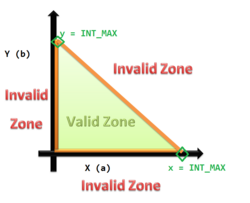
Boundary values (drawn only for the overflow case) are being shown as the orange line in the right hand side figure.

For another example, if the input values were months of the year, expressed as integers, the input parameter 'month' might have the following partitions:

       ... -2 -1  0 1 .............. 12 13  14  15 .....
     --------------|-------------------|-------------------
invalid partition 1   valid partition   invalid partition 2

The boundary between two partitions is the place where the behavior of the application changes and is not a real number itself. The boundary value is the minimum (or maximum) value that is at the boundary. The number 0 is the maximum number in the first partition, the number 1 is the minimum value in the second partition, both are boundary values. Test cases should be created to generate inputs or outputs that will fall on and to either side of each boundary, which results in two cases per boundary. The test cases on each side of a boundary should be in the smallest increment possible for the component under test, for an integer this is 1, but if the input was a decimal with 2 places then it would be .01. In the example above there are boundary values at 0,1 and 12,13 and each should be tested.

Boundary value analysis does not require invalid partitions. Take an example where a heater is turned on if the temperature is 10 degrees or colder. There are two partitions (temperature≤10, temperature>10) and two boundary values to be tested (temperature=10, temperature=11).

Where a boundary value falls within the invalid partition the test case is designed to ensure the software component handles the value in a controlled manner. Boundary value analysis can be used throughout the testing cycle and is equally applicable at all testing phases.

External links

• The Testing Standards Working Party website.

References

- ↑ Craig, Rick David; Jaskiel, Stefan P. (2002). Systematic Software Testing. Artech House. pp. 155–156. ISBN 9781580537926. https://books.google.com/books?id=2_gbZYZcZXgC. Retrieved February 25, 2024.