Common spatial pattern

Two sets of overlapping data used to illustrate how CSP can separate the data.

Two sets of data after rotation by CSP to maximize the ratio of the variances along the two axes.

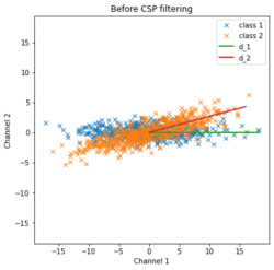
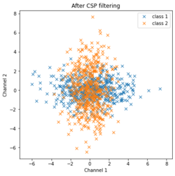
Common spatial pattern (CSP) is a mathematical procedure used in signal processing for separating a multivariate signal into additive subcomponents which have maximum differences in variance between two windows.

Details

Let [math]\displaystyle{ \mathbf{X}_1 }[/math] of size [math]\displaystyle{ (n,t_1) }[/math] and [math]\displaystyle{ \mathbf{X}_2 }[/math] of size [math]\displaystyle{ (n,t_2) }[/math] be two windows of a multivariate signal, where [math]\displaystyle{ n }[/math] is the number of signals and [math]\displaystyle{ t_1 }[/math] and [math]\displaystyle{ t_2 }[/math] are the respective number of samples.

The CSP algorithm determines the component [math]\displaystyle{ \mathbf{w}^\text{T} }[/math] such that the ratio of variance (or second-order moment) is maximized between the two windows:

[math]\displaystyle{ \mathbf{w}={\arg \max}_\mathbf{w} \frac{ \left\| \mathbf{wX}_1 \right\| ^2 } { \left\| \mathbf{wX}_2 \right\| ^2 } }[/math]

The solution is given by computing the two covariance matrices:

[math]\displaystyle{ \mathbf{R}_1=\frac{\mathbf{X}_1\mathbf{X}_1^\text{T}}{t_1} }[/math]

[math]\displaystyle{ \mathbf{R}_2=\frac{\mathbf{X}_2\mathbf{X}_2^\text{T}}{t_2} }[/math]

Then, the simultaneous diagonalization of those two matrices (also called generalized eigenvalue decomposition) is realized. We find the matrix of eigenvectors [math]\displaystyle{ \mathbf{P}=\begin{bmatrix} \mathbf{p}_1 & \cdots & \mathbf{p}_n \end{bmatrix} }[/math] and the diagonal matrix [math]\displaystyle{ \mathbf{D} }[/math] of eigenvalues [math]\displaystyle{ \{\lambda_1, \cdots , \lambda_n \} }[/math] sorted by decreasing order such that:

[math]\displaystyle{ \mathbf{P}^{\mathrm{T}} \mathbf{R}_1 \mathbf{P} = \mathbf{D} }[/math]

and

[math]\displaystyle{ \mathbf{P}^{\mathrm{T}} \mathbf{R}_2 \mathbf{P} = \mathbf{I}_n }[/math]

with [math]\displaystyle{ \mathbf{I}_n }[/math] the identity matrix.

This is equivalent to the eigendecomposition of [math]\displaystyle{ \mathbf{R}_2^{-1} \mathbf{R}_1 }[/math]:

[math]\displaystyle{ \mathbf{R}_2^{-1} \mathbf{R}_1=\mathbf{PDP}^{-1} }[/math]

[math]\displaystyle{ \mathbf{w}^\text{T} }[/math] will correspond to the first column of [math]\displaystyle{ \mathbf{P} }[/math]:

[math]\displaystyle{ \mathbf{w}=\mathbf{p}_1^\text{T} }[/math]

Discussion

Relation between variance ratio and eigenvalue

The eigenvectors composing [math]\displaystyle{ \mathbf{P} }[/math] are components with variance ratio between the two windows equal to their corresponding eigenvalue:

[math]\displaystyle{ \mathbf{\lambda}_i = \frac{ \left\| \mathbf{p}_i^\text{T} \mathbf{X}_1 \right\| ^2 }{ \left\| \mathbf{p}_i^\text{T} \mathbf{X}_2 \right\| ^2 } }[/math]

Other components

The vectorial subspace [math]\displaystyle{ E_i }[/math] generated by the [math]\displaystyle{ i }[/math] first eigenvectors [math]\displaystyle{ \begin{bmatrix} \mathbf{p}_1 & \cdots & \mathbf{p}_i \end{bmatrix} }[/math] will be the subspace maximizing the variance ratio of all components belonging to it:

[math]\displaystyle{ E_i={\arg \max}_{E} \begin{pmatrix}\min_{p \in E} \frac{ \left\| \mathbf{p^\text{T} X}_1 \right\| ^2 }{ \left\| \mathbf{p^\text{T} X}_2 \right\| ^2}\end{pmatrix} }[/math]

On the same way, the vectorial subspace [math]\displaystyle{ F_j }[/math] generated by the [math]\displaystyle{ j }[/math] last eigenvectors [math]\displaystyle{ \begin{bmatrix} \mathbf{p}_{n-j+1} & \cdots & \mathbf{p}_n \end{bmatrix} }[/math] will be the subspace minimizing the variance ratio of all components belonging to it:

[math]\displaystyle{ F_j = {\arg \min}_{F} \begin{pmatrix}\max_{p \in F} \frac{ \left\| \mathbf{p^\text{T} X}_1 \right\| ^2 }{ \left\| \mathbf{p^\text{T} X}_2 \right\| ^2} \end{pmatrix} }[/math]

Variance or second-order moment

CSP can be applied after a mean subtraction (a.k.a. "mean centering") on signals in order to realize a variance ratio optimization. Otherwise CSP optimizes the ratio of second-order moment.

Choice of windows X₁ and X₂

• The standard use consists on choosing the windows to correspond to two periods of time with different activation of sources (e.g. during rest and during a specific task).
• It is also possible to choose the two windows to correspond to two different frequency bands in order to find components with specific frequency pattern. Those frequency bands can be on temporal or on frequential basis. Since the matrix [math]\displaystyle{ \mathbf{P} }[/math] depends only of the covariance matrices, the same results can be obtained if the processing is applied on the Fourier transform of the signals.
• Y. Wang has proposed a particular choice for the first window [math]\displaystyle{ \mathbf{X}_1 }[/math] in order to extract components which have a specific period. [math]\displaystyle{ \mathbf{X}_1 }[/math] was the mean of the different periods for the examined signals.
• If there is only one window, [math]\displaystyle{ \mathbf{R}_2 }[/math] can be considered as the identity matrix and then CSP corresponds to Principal component analysis.

Relation between LDA and CSP

Linear discriminant analysis (LDA) and CSP apply in different circumstances. LDA separates data that have different means, by finding a rotation that maximizes the (normalized) distance between the centers of the two sets of data. On the other hand, CSP ignores the means. Thus CSP is good, for example, in separating the signal from the noise in an event-related potential (ERP) experiment because both distributions have zero mean and there is no distinction for LDA to separate. Thus CSP finds a projection that makes the variance of the components of the average ERP as large as possible so the signal stands out above the noise.

Applications

The CSP method can be applied to multivariate signals in generally, is commonly found in application to electroencephalographic (EEG) signals. Particularly, the method is often used in brain–computer interfaces to retrieve the component signals which best transduce the cerebral activity for a specific task (e.g. hand movement). It can also be used to separate artifacts from EEG signals.

CSP can be adapted for the analysis of the event-related potentials.

See also

• Blind signal separation

References

- ↑ Zoltan J. Koles, Michael S. Lazaret and Steven Z. Zhou, "Spatial patterns underlying population differences in the background EEG", Brain topography, Vol. 2 (4) pp. 275-284, 1990
- ↑ 2.0 2.1 S. Boudet, "Filtrage d'artefacts par analyse multicomposantes de l'électroencephalogramme de patients épileptiques.", PhD. Thesis: Unviversité de Lille 1, 07/2008
- ↑ Y. Wang, "Reduction of cardiac artifacts in magnetoencephalogram." Proc. of the 12th Int. Conf. on Biomagnetism, 2000
- ↑ G. Pfurtscheller, C. Guger and H. Ramoser "EEG-based brain-computer interface using subject-specific spatial filters", Engineering applications of bio-inspired artificial neural networks, Lecture Notes in Computer Science, 1999, Vol. 1607/1999, pp. 248-254
- ↑ M. Congedo, L. Korczowski, A. Delorme and F. Lopes da Silva, "Spatio-temporal common pattern: A companion method for ERP analysis in the time domain", Journal of Neuroscience Methods, Vol. 267, pp. 74-88, 2016