Deriche edge detector

Deriche edge detector is an edge detection operator developed by Rachid Deriche in 1987. It is a multistep algorithm used to obtain an optimal result of edge detection in a discrete two-dimensional image. This algorithm is based on John F. Canny's work related to the edge detection (Canny's edge detector) and his criteria for optimal edge detection:

Detection quality – all existing edges should be marked and no false detection should occur.
Accuracy - the marked edges should be as close to the edges in the real image as possible.
Unambiguity - a given edge in the image should only be marked once. No multiple responses to one edge in the real image should occur.

For this reason, this algorithm is often referred to as Canny-Deriche detector.

Differences between Canny and Deriche edge detector

Deriche edge detector, like Canny edge detector, consists of the following 4 steps:

Smoothing
Calculation of magnitude and gradient direction
Non-maximum suppression
Hysteresis thresholding (using two thresholds)

The essential difference is in the implementation of the first two steps of the algorithm. Unlike the Canny edge detector, Deriche edge detector uses the IIR filter in the form:

[math]\displaystyle{ f(x)=\frac{S}{\omega}e^{-\alpha|x|}\sin\omega x }[/math]

The filter optimizes the Canny criteria. As is evident from the preceding formula, the most effective filter is obtained when the value of [math]\displaystyle{ \omega }[/math] approaches 0. Such filter then uses the formula:

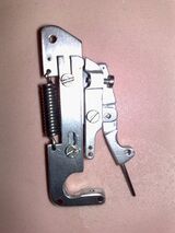
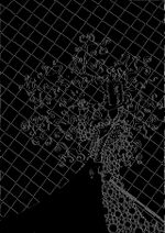
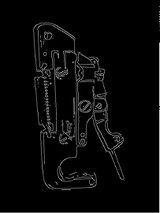
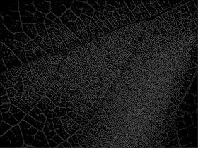
[math]\displaystyle{ f(x)=Sxe^{-\alpha|x|} }[/math]

The advantage of such a filter is that it can be adapted to the characteristics of the processed image using only one parameter. If the value of α is small (usually between 0.25 and 0.5), it results in better detection. On the other hand, better localization is achieved when the parameter has a higher value (around 2 or 3). For most of the normal cases parameter value of around 1 is recommended.

Example of smoothing using Deriche filter
Image
α	α = 0.25	α = 0.5	α = 1	α = 2

Using the IIR filter makes sense especially in cases where the processed image is noisy or a large amount of smoothing is required (which leads to large convolution kernel for FIR filter). In these cases, the Deriche detector has considerable advantage over the Canny detector, because it is able to process images in a short constant time independent of the desired amount of smoothing.

Deriche detector implementation

It is possible to separate the process of obtaining the value of a two-dimensional Deriche filter into two parts. In first part, image array is passed in the horizontal direction from left to right according to the following formula:

[math]\displaystyle{ y_{ij}^1=a_1x_{ij}+a_2x_{ij-1}+b_1y_{ij-1}^1+b_2y_{ij-2}^1 }[/math]

and from right to left according to the formula:

[math]\displaystyle{ y_{ij}^2=a_3x_{ij+1}+a_4x_{ij+2}+b_1y_{ij+1}^2+b_2y_{ij+2}^2 }[/math]

The result of the computation is then stored into temporary two-dimensional array:

[math]\displaystyle{ \theta_{ij}=c_1(y_{ij}^1+y_{ij}^2) }[/math]

The second step of the algorithm is very similar to the first one. The two-dimensional array from the previous step is used as the input. It is then passed in the vertical direction from top to bottom and bottom-up according to the following formulas:

[math]\displaystyle{ y_{ij}^1=a_5\theta_{ij}+a_6\theta_{i-1j}+b_1y_{i-1j}^1+b_2y_{i-2j}^1 }[/math]

[math]\displaystyle{ y_{ij}^2=a_7\theta_{i+1j}+a_8\theta_{i+2j}+b_1y_{i+1j}^2+b_2y_{i+2j}^2 }[/math]

[math]\displaystyle{ \Theta_{ij}=c_2(y_{ij}^1+y_{ij}^2) }[/math]

The description of the algorithm implies that the processed rows and columns are independent of each other. As a result, the solution based on the IIR filter is often employed in embedded systems and architectures which support a high level of parallelization.

Deriche filter coefficients
	smoothing	x-derivative	y-derivative
[math]\displaystyle{ k }[/math]	[math]\displaystyle{ \frac{{(1-e^{-\alpha})}^2}{1+2\alpha e^{-\alpha}-e^{-2\alpha}} }[/math]	[math]\displaystyle{ \frac{{(1-e^{-\alpha})}^2}{1+2\alpha e^{-\alpha}-e^{-2\alpha}} }[/math]	[math]\displaystyle{ \frac{{(1-e^{-\alpha})}^2}{1+2\alpha e^{-\alpha}-e^{-2\alpha}} }[/math]
[math]\displaystyle{ a_1 }[/math]	[math]\displaystyle{ k }[/math]	0	[math]\displaystyle{ k }[/math]
[math]\displaystyle{ a_2 }[/math]	[math]\displaystyle{ ke^{-\alpha}(\alpha-1) }[/math]	1	[math]\displaystyle{ ke^{-\alpha}(\alpha-1) }[/math]
[math]\displaystyle{ a_3 }[/math]	[math]\displaystyle{ ke^{-\alpha}(\alpha+1) }[/math]	-1	[math]\displaystyle{ ke^{-\alpha}(\alpha+1) }[/math]
[math]\displaystyle{ a_4 }[/math]	[math]\displaystyle{ -ke^{-2\alpha} }[/math]	0	[math]\displaystyle{ -ke^{-2\alpha} }[/math]
[math]\displaystyle{ a_5 }[/math]	[math]\displaystyle{ k }[/math]	[math]\displaystyle{ k }[/math]	0
[math]\displaystyle{ a_6 }[/math]	[math]\displaystyle{ ke^{-\alpha}(\alpha-1) }[/math]	[math]\displaystyle{ ke^{-\alpha}(\alpha-1) }[/math]	1
[math]\displaystyle{ a_7 }[/math]	[math]\displaystyle{ ke^{-\alpha}(\alpha+1) }[/math]	[math]\displaystyle{ ke^{-\alpha}(\alpha+1) }[/math]	-1
[math]\displaystyle{ a_8 }[/math]	[math]\displaystyle{ -ke^{-2\alpha} }[/math]	[math]\displaystyle{ -ke^{-2\alpha} }[/math]	0
[math]\displaystyle{ b_1 }[/math]	[math]\displaystyle{ 2e^{-\alpha} }[/math]	[math]\displaystyle{ 2e^{-\alpha} }[/math]	[math]\displaystyle{ 2e^{-\alpha} }[/math]
[math]\displaystyle{ b_2 }[/math]	[math]\displaystyle{ -e^{-2\alpha} }[/math]	[math]\displaystyle{ -e^{-2\alpha} }[/math]	[math]\displaystyle{ -e^{-2\alpha} }[/math]
[math]\displaystyle{ c_1 }[/math]	1	[math]\displaystyle{ -{(1-e^{-\alpha})}^2 }[/math]	1
[math]\displaystyle{ c_2 }[/math]	1	1	[math]\displaystyle{ -{(1-e^{-\alpha})}^2 }[/math]

The mathematical properties of the algorithm are often used in practical implementation of the Deriche detector. It is sufficient to implement only one part of the algorithm, which is then called twice, while performing a transposition of the resulting matrix.

Examples of using Deriche filter on various source images
Source image
Filtered image
Filter parameters	α = 1.5 low threshold = 20 high threshold = 40	α = 4.0 low threshold = 50 high threshold = 90	α = 0.8 low threshold = 26 high threshold = 41	α = 1.0 low threshold = 15 high threshold = 35